Getting Started with Python

Getting Started with Python#

In this tutorial, we go through basic commands in python. Let’s start with a simple command in Python.

print('Hello World')

Hello World

Certainly, we can create more complex commands using print() that interested readers can find some of them here.

1. Packages#

1.1 Installing Packages#

Packages are an essential part of python that can make tasks easier for users. We can use the following syntax to install packages:

pip install packagename

Example: Installing numpy package.

pip install numpy

Moreover, this can be done through Conda Terminal using the following syntax:

conda install numpy

To see available packages using conda environment, one can search using

conda search packagename

Moreover, to see channels, we can use

conda config --show channels

Also, to add a new channel to the bottom of the channel list

conda config --append channels channelname

For example, we can add conda-forge to the bottom of the channel list

conda config --append channels conda-forge

Similarly, to add a new channel to the top of the channel list

For example, we can add conda-forge to the top of the channel list

conda config --add channels conda-forge 

See managing channels for more details.

1.2 Importing Packages#

Some useful package:

NumPy: a package for computation and it includes a variety of tools from basic algebra to managing data.
Pandas: a package that is used to create a data frame using imported data (from user or URL). This package is crucial for data analysis.
SciPy: a package for math, science, and engineering. It includes tools for optimization, linear algebra, integration, and many more.
Plotly: It is used for visualization and creating two-dimensional and three-dimensional graphs.

One can import all contents of a package or import a particular part of it. We recommend importing packages using the “as” feature (see blew for details). This allows importing many packages without being worried about any overlapping.

Importing the contents of the package or module *abc. Syntax:

import abc

Importing only module or subpackage xyz from another package or module abc. Syntax:

from abc import xyz

To assign an imported package or module abc as other_name. Syntax:

import abc as other_name

Example:

## import numpy pcckage
import numpy
numpy.pi

3.141592653589793

## from numpy pcckage import everything
from numpy import *
## * means import everything
pi

3.141592653589793

## import abc as other_name
import numpy as np
np.pi

3.141592653589793

2. Control Flow#

Control flow includes Conditional statements, loops, branching, …

2.1. if Statements#

We can use the following syntex to use if, elif and else.

Syntax:

if expression:
    statements
elif expression:
    statements
else:
    statements
end

Example: Checking wheter a given number \(x\) is smaller than 10, equal 10 or greater than 10.

## given number x
x = 10;
## Checking wheter a given number  x  is smaller than 10, equal 10 or greater than 10
if x<10:
    print('X is smaller than 10')
elif x==10:
    print('X is equal 10')
else:
    print('X is greater than 10')

X is equal 10

Example: Checking wheter given number \(x\) and \(y\) are smaller than 10, greater than 10 or none of above.

## given nubmers x and y
x=11;y=9;
## Checking wheter given number  x and y are smaller than 10, greater than 10 or none of above.
if (x>10) & (y<10):
    print('x>10 & y<10')
elif (x<=10) & (y<10):
    print('x<=10 & y<10')
elif (x<=10) & (y>=10):
    print('x<=10 & y>=10')
else:
    print('None of above')

x>10 & y<10

2.2. Loops#

Loops are used for iterating a process. Two popular loops are for and while loops.

2.2.1. for loops#

for loop is used to repeat some statements for a specified number of times.

Syntax:

for index in values:
    statements

Example: Let’s generate the following sequence using Python

\[\begin{align*} \{ 0, 1, 3, 6, 10, \ldots\} \end{align*}\]

## the first 10 elements of the sequence
S=0;N=10;
for i in range(0,N):
    S+=i
    print("S_%d=%d" % (i,S))

S_0=0
S_1=1
S_2=3
S_3=6
S_4=10
S_5=15
S_6=21
S_7=28
S_8=36
S_9=45

To loop over a sequence in reverse, first specify the sequence in a forward direction and then call the reversed() function.

Example:

N=5;
for i in reversed(range(0,N)):
    S=i
    print("S_%d=%d" % (i,S))

S_4=4
S_3=3
S_2=2
S_1=1
S_0=0

2.2.2. Nested loops#

Implementing a loop inside another loop is called a nested loop. For example, we can

for loop: ## Outer loop
    [doing something using the outer loop iteration]  ## Optional
    for loop:   ## Nested loop
        [doing something using nested loop iteration]

Example:

for i in range(1,3):
    for j in range(1,4):
        print("%d+%d=%d" % (i,j,i+j))

1+1=2
1+2=3
1+3=4
2+1=3
2+2=4
2+3=5

Note: the the second loops runs first.

Example:

num_list = [1, 2, 3]
alpha_list = ['a', 'b', 'c']

for N in num_list:
    for L in alpha_list:
        print("%s and %d" % (L,N))

a and 1
b and 1
c and 1
a and 2
b and 2
c and 2
a and 3
b and 3
c and 3

2.2.3. While loops#

while loop is used to repeat some statements when condition is true

Syntax:

while expression:
    statements

Example:

n = 100

s = 0
counter = 1
while counter <= n:
    s = s + counter
    counter += 1

print("Sum of 1 until %d: %d" % (n,s))

Sum of 1 until 100: 5050

We can generate the sequnece \(\{ 0, 1, 3, 6, 10, \ldots\}\) using while loop as well.

## the first 10 elements of the sequence
S=0;N=10;i=0;
while i<N:
    S+=i
    print("S_%d=%d" % (i,S))
    i+=1;

S_0=0
S_1=1
S_2=3
S_3=6
S_4=10
S_5=15
S_6=21
S_7=28
S_8=36
S_9=45

2.2.4. break#

[source python.org]

The break statement, like in C, breaks out of the innermost enclosing for or while loop.

Loop statements may have an else clause; it is executed when the loop terminates through exhaustion of the list (with for) or when the condition becomes false (with while), but not when the loop is terminated by a break statement.

Example:

for i in range(1,3):
    for j in range(1,4):
        if i+j==5:
            break
        else:
            print("%d+%d=%d" % (i,j,i+j))

1+1=2
1+2=3
1+3=4
2+1=3
2+2=4

Example:

for i in range(1,3):
    for j in range(1,4):
        if i+j!=5:
            continue
        else:
            print("%d+%d=%d" % (i,j,i+j))

2+3=5

3. Defining a Function#

Syntax

def functionname( parameters ):
    "function_docstring"
    function_suite
    return [expression]

Example:

def Add3( x ):
    "This function adds 3 to x"
    print (x+3)
    return

## x=1 
Add3(1),
## x=2
Add3(2)

4
5

3.1. functions with two arguments#

def printinfo( name, age = 35 ):
  ## print name
    print ("Name: ", name)
    ## print age. If age is not defined, the default value is 35.
    print ("Age ", age)
    return

printinfo( age = 50, name = "Henry" )
printinfo( name = "Henry" )

Name:  Henry
Age  50
Name:  Henry
Age  35

Example: the following function takes \(x\) and \(y\) and retruns \(x^2\) and \(y^2\).

## the following function takes x and y and retruns x^2 and y^2.
def square(x,y):
    return x*x, y*y

x2, y2 = square(3,10)
print(x2)
print(y2) 

9
100

4. Plots#

4.1. Pyplot#

Pyplot from matplotlib (i.e. matplotlib.pyplot) provides a wide variety of function that can be compared with MATLAB plot functions.

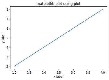
Example: Let’s plot a line using \(\{(1,2),(2,4),(3,6),(4,8)\}\).

import matplotlib.pyplot as plt
## define X
X=[1,2,3,4]
## define Y
Y=[2,4,6,8]
## ploting (X,Y)
plt.plot(X,Y)
plt.xlabel('x label')
plt.ylabel('y label')
plt.title('matplotlib plot using plot')
plt.show()

_images/6c6fa46a09cd04cd02f47014b9231de8562cb6eabfb869c52853250447a6a069.png

We also can use the following command to use plot

from matplotlib.pyplot import *
X=[1,2,3,4];Y=[2,4,6,8];
plot(X,Y)
xlabel('x label'),ylabel('y label'),title('matplotlib plot using plot')
show()

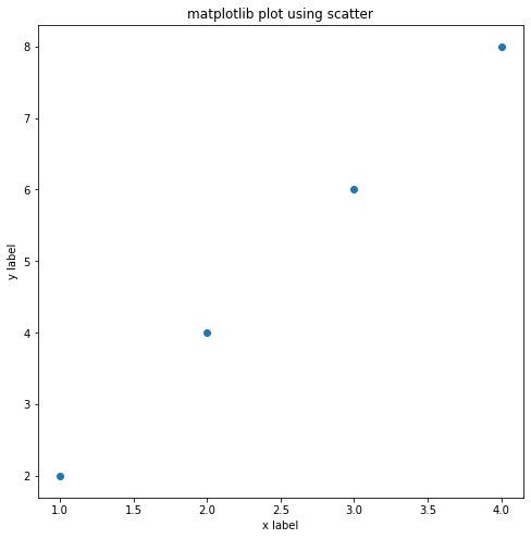
We also can use scatter to plot discrete data. For Example,

import matplotlib.pyplot as plt
X=[1,2,3,4]
Y=[2,4,6,8]
## Figure size is Figure size 800x800 with 1 Axes
plt.figure(figsize = (8, 8))
plt.scatter(X,Y)
plt.xlabel('x label')
plt.ylabel('y label')
plt.title('matplotlib plot using scatter')
plt.show()

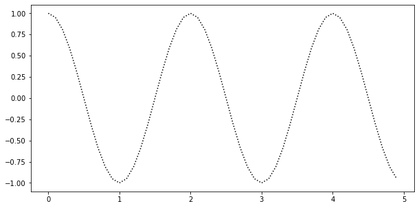
_images/69a24efd3dba06979d1b4e85c91f24494557a716740da203b1e55b2bae730e98.png

Example: Let’s plot \(\cos(\pi t)\) with \(0\leq t \leq 5\)

import numpy as np
import matplotlib.pyplot as plt

#### definining a function
def f(t):
    return np.cos(np.pi*t)
## discretizing [0,5] with dh=0.1
t = np.arange(0.0, 5.0, 0.1)
plt.figure(figsize = (10, 5))
plt.plot(t, f(t), 'k:')

[<matplotlib.lines.Line2D at 0x2200aae6b50>]

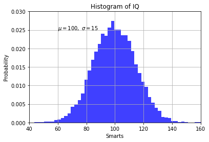
_images/0d4a090daa32406ec1092c1852c34089be5204cf0466c573446e6ac0d8480e31.png

The hist() function automatically generates histograms and returns the bin counts or probabilities.

Example: The hist() function automatically generates histograms and returns the bin counts or probabilities.

import numpy as np
import matplotlib.pyplot as plt

## Fixing random state for reproducibility
np.random.seed(19680801)

mu, sigma = 100, 15
## random.randn(10000) creates a random array with the size of 10000
x = mu + sigma * np.random.randn(10000)

## the histogram of the data
n, bins, patches = plt.hist(x, 50, density=True, facecolor='b', alpha=0.75)


plt.xlabel('Smarts')
plt.ylabel('Probability')
plt.title('Histogram of IQ')

plt.text(60, .025, r'$\mu=100,\ \sigma=15$')
plt.axis([40, 160, 0, 0.03])
plt.grid(True)
plt.show()

_images/69685ef169d3a0a0c78083ce9cc6772472ee7daed8c2e43b845e66f7f6ebf4e9.png

4.2. subplot#

Sometimes, it is more convenient to include more than one plot in a figure. Doins so, we can use subplot.

import numpy as np
import matplotlib.pyplot as plt

## defining a function using lambda (simlar to @ in MATLAB)
f= lambda t : np.exp(-t)*np.cos(np.pi*t)
## discretizing
t1 = np.arange(0.0, 5.0, 0.1)
t2 = np.arange(0.0, 5.0, 0.02)

plt.subplots(figsize = (10, 5))
## The first subplot
plt.subplot(211)
plt.plot(t1, f(t1), 'bo', t2, f(t2), 'k')
plt.grid()
## The second subplot is plotting cos(2*np.pi*t2) but we do this using a different approach than the first one
plt.subplot(212)
plt.plot(t2, np.cos(2*np.pi*t2), 'r--')
plt.grid()
plt.show()

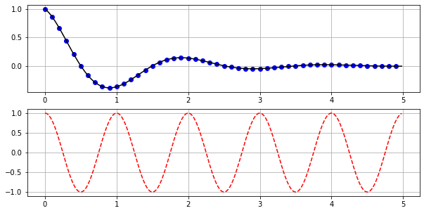
_images/e4db2965ae4f4d8d599629d846bb6922af70138d96d35125cb33a984150ee818.png

An alternative way can be considered as follows:

fig, ax = plt.subplots(nrows=2, ncols=1, figsize=(10, 5), sharex=False)
_ = ax[0].plot(t1, f(t1), 'bo', t2, f(t2), 'k')
_ = ax[0].grid()
_ = ax[1].plot(t2, np.cos(2*np.pi*t2), 'r--')
_ = ax[1].grid()

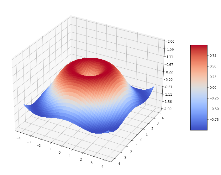
4.3. Three-dimensional plotting#

We can use mplot3d from mpl_toolkits to generate 3D plots.

Example: For example, let’s plot \(z=x^2+y^2\) with \(-4\leq x,y\leq 4\).

from mpl_toolkits.mplot3d import Axes3D

import matplotlib.pyplot as plt
from matplotlib import cm
from matplotlib.ticker import LinearLocator, FormatStrFormatter
import numpy as np


fig = plt.figure(figsize = (20, 10))
ax = fig.add_subplot(111, projection='3d')

## Make data.
X = np.arange(-4, 4, 0.02)
Y = np.arange(-4, 4, 0.02)
X, Y = np.meshgrid(X, Y)
R = np.sqrt(X**2 + Y**2)
Z = np.sin(R)

## Plot the surface.
surf = ax.plot_surface(X, Y, Z, cmap=cm.coolwarm,
                       linewidth=0, antialiased=False)

## Customize the z axis.
ax.set_zlim(-2.00, 2.00)
ax.zaxis.set_major_locator(LinearLocator(10))
ax.zaxis.set_major_formatter(FormatStrFormatter('%.02f'))

## Add a color bar which maps values to colors.
fig.colorbar(surf, shrink=0.5, aspect=5)

plt.show()

_images/df4e29d4c58da107e9d5dedac7058c26d4c6765e1a748988f6dd629d1a24bcf0.png

For more examples of plots, please check here.

5. Symbolic computations in Python#

Let us define a symbolic expression and appy some useful functions on it [source].

Function	Description
expand(expr)	expands the arithmetical expression expr.
simplify(expr)	transforms an expression into a simpler form.
factor(expr)	Factors a polynomial into irreducible polynomials.
diff(func, var, n)	Returns nth derivative of func .
integrate(func, var)	Evaluates Indefinite integral
integrate(func, (var, a, b))	Evaluates Definite integral
limit(function, variable, point)	Evaluates Limit of symbolic expression.
series(expr, var, point, order)	Taylor series of an expression at a point.
solve	Equations and systems solver.
dsolve	solves differential equations.

from sympy import *
x, y = symbols('x y')

Example: (expand, simplify and factor)

## expand
f = x**2 + 2*x*y
print("f^2=%s" % (f*f))
print("expand = %s" % expand(f*f))
print("simplify = %s" % simplify(f*f))
print("factor = %s" % factor(f*f))

f^2=(x**2 + 2*x*y)**2
expand = x**4 + 4*x**3*y + 4*x**2*y**2
simplify = x**2*(x + 2*y)**2
factor = x**2*(x + 2*y)**2

Example: (diff)

print("f=%s" % (f))
print("f_x=%s" % diff(f, x))
print("f_y=%s" % diff(f, y))
print("f_xx=%s" % diff(f, x, 2))
print("f_yx=%s" % diff(diff(f, y),x))

f=x**2 + 2*x*y
f_x=2*x + 2*y
f_y=2*x
f_xx=2
f_yx=2

Example: (integrate)

print("f=%s" % (f))
print("Indefinite integral (with respect to x) = %s" % integrate(f, x))
print("Indefinite integral (with respect to y) = %s" % integrate(f, y))

print("Definite integral (with respect to x on [2,3]) = %s" % integrate(f, (x,2,3)))
print("Definite integral (with respect to y on [2,3]) = %s" % integrate(f, (y,2,3)))

f=x**2 + 2*x*y
Indefinite integral (with respect to x) = x**3/3 + x**2*y
Indefinite integral (with respect to y) = x**2*y + x*y**2
Definite integral (with respect to x on [2,3]) = 5*y + 19/3
Definite integral (with respect to y on [2,3]) = x**2 + 5*x

Example: Let’s compute

(a) \(\int_{-\infty}^\infty \sin{(x^2)}\,dx\)
(b) \(\lim_{x\to 0}\frac{\sin{(x)}}{x}\)
(c) \(\lim_{x\to -\infty}\exp(x)\)

#### a
print("a=%s" % integrate(sin(x**2), (x, -oo, oo)))
#### b
print("b=%s" % limit(sin(x)/x, x, 0))
#### c
print("c=%s" % limit(exp(x), x, -oo))

a=sqrt(2)*sqrt(pi)/2
b=1
c=0

Example: Evaluate Taylor series of

(a) \(\sin(x)\) at \(x=0\)
(a) \(\cos(x)\) at \(x=1\)

#### a
print("(a) Taylor series of sin(x) at x=0 : %s " % series(sin(x), x))
#### b
print("(b) Taylor series of cos(x) at x=0 : %s " % series(cos(x), x, 1, 3))

(a) Taylor series of sin(x) at x=0 : x - x**3/6 + x**5/120 + O(x**6) 
(b) Taylor series of cos(x) at x=0 : cos(1) - (x - 1)*sin(1) - (x - 1)**2*cos(1)/2 + O((x - 1)**3, (x, 1)) 

Example: Let’s solve the following equations

(a) \(x^3-1=0\) for \(x\)
(b) \(x+y=2\) for \(y\)

solve(x**3 - 1, x)

[1, -1/2 - sqrt(3)*I/2, -1/2 + sqrt(3)*I/2]

solve(x+y-2, y)

[2 - x]

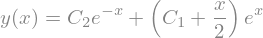
Example: Let’s solve the differential equation \(y'' - y = e^x\).

#### displaying the soltuion in laTex format
init_printing(use_unicode=True)
##
from sympy import Function, dsolve, Eq, Derivative, sin, cos, symbols
from sympy.abc import x
y = Function('y')
dsolve(Derivative(y(x), x, x) -y(x)-exp(x), y(x))

_images/0eebf7c4f07731afd7224566292df5fb3f0ddf284e383e006fcadfb3b759d716.png

We also can find the eigenvalues of a marix using Python

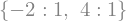
Example: Matrices

Matrix([[1, 3], [3, 1]]).eigenvals()

_images/7a44fe5fed169b21566d258d18f09ab30cb50a4a858ccd6acceead97da02068b.png

x, y = symbols('x y')
Matrix([[0,x*x], [y*y,0]]).eigenvals()

_images/8628082a91fe5e83b2dce591f81b60cf9fb3974cedd7201cf0a6ea53b2cb33b8.png

Finally, we can print outputs in \(\LaTeX\) format.

Example:

latex(Integral(cos(x)**2, (x, 0, pi)))

'\\int\\limits_{0}^{\\pi} \\cos^{2}{\\left(x \\right)}\\, dx'

6. Data Structures#

6.1. Lists#

Syntax	Description
list.append(x)	Add an item to the end of a list.
list.extend(iterable)	Extend a list by appending all the items from the iterable.
list.insert(i, x)	Insert an item at a given position of a list.
list.remove(x)	Remove the first item from a list whose value is equal to x.
list.pop([i])	Remove the item at the given position in a list, and return it.
list.clear()	Remove all items from a list.
list.index(x[, start[, end]])	Return zero-based index in a list of the first item whose value is equal to x.
list.count(x)	Return the number of times x appears in the list
list.sort(key=None, reverse=False)	Sort the items of the list in place.
list.reverse()	Reverse the elements of the list in place.
list.copy()	Return a shallow copy of the list.

Here are all of the methods of list objects (source):

Example:

L=list(range(1,4))
print('L = %s' % L)
print('append: Add 5 to the end of a list.')
L.append(5)
print('L = %s' % L)
print('extend: Extend a list by appending [6,7].')
L.extend([6,7])
print('L = %s' % L)
print('insert: Insert 0 at position 0 of a list.')
L.insert(0, 0)
print('L = %s' % L)
print('insert: Insert 1.5 at position 2 of a list.')
L.insert(2, 1.5)
print('L = %s' % L)
print('remove: remove 2 from the list')
L.remove(2)
print('L = %s' % L)
print('remove: remove 1 from the list')
L.remove(1)
print('L = %s' % L)

L = [1, 2, 3]
append: Add 5 to the end of a list.
L = [1, 2, 3, 5]
extend: Extend a list by appending [6,7].
L = [1, 2, 3, 5, 6, 7]
insert: Insert 0 at position 0 of a list.
L = [0, 1, 2, 3, 5, 6, 7]
insert: Insert 1.5 at position 2 of a list.
L = [0, 1, 1.5, 2, 3, 5, 6, 7]
remove: remove 2 from the list
L = [0, 1, 1.5, 3, 5, 6, 7]
remove: remove 1 from the list
L = [0, 1.5, 3, 5, 6, 7]

Example:

L=list(range(1,5))
print('L = %s' % L)
print('The first item of the list is %s' % L.pop(0))
print('The second item of the list is %s' % L.pop(0))
print('The last item of the list is %s' % L.pop())

L = [1, 2, 3, 4]
The first item of the list is 1
The second item of the list is 2
The last item of the list is 4

L=list(range(1,5))
print('L = %s' % L)
print('Remove all items from a list:')
print('Using L.clear: %s' % L.clear())

L = [1, 2, 3, 4]
Remove all items from a list:
Using L.clear: None

Example:

L=list(range(1,10))
print('L =  % s' % L)
print('the index of the first item whose value is equal to 5 is % s' % L.index(5))

L =  [1, 2, 3, 4, 5, 6, 7, 8, 9]
the index of the first item whose value is equal to 5 is 4

Example:

L=[1, 1, 2, 5, 15, 3, 4]
print('L =  % s' % L)
print('the number of times 1 appears in the list = %s' % L.count(1))
L.sort(key=None, reverse=False)
print('Sort the items of the list in place : %s' % L)
L.reverse()
print('Reverse the elements of the list in place : %s' % L)
print('a copy of L = %s' % L.copy())

L =  [1, 1, 2, 5, 15, 3, 4]
the number of times 1 appears in the list = 2
Sort the items of the list in place : [1, 1, 2, 3, 4, 5, 15]
Reverse the elements of the list in place : [15, 5, 4, 3, 2, 1, 1]
a copy of L = [15, 5, 4, 3, 2, 1, 1]

Example:

fruits = ['Apricots','Avocado','Watermelon','Strawberries','Orange', 'Apple', 'Banana', 'Kiwi', 'Apple', 'Strawberries']
#### Count
print("The number of Strawberries = %i" % fruits.count('Strawberries'))
print("The number of Watermelon = %i" % fruits.count('Watermelon'))

The number of Strawberries = 2
The number of Watermelon = 1

#### Find
fruits.index('Watermelon', 1)  ## Find next banana starting a position 1

_images/d09c16c60c1bec6d87b5a6ea36a28d98601be002bd4b459592b55e0896ad9754.png

## Reverse the elements of the list in place.
fruits.reverse()
fruits

['Strawberries',
 'Apple',
 'Kiwi',
 'Banana',
 'Apple',
 'Orange',
 'Strawberries',
 'Watermelon',
 'Avocado',
 'Apricots']

## Add 'Pomegranate' to the end of the list
fruits.append('Pomegranate')
fruits

['Strawberries',
 'Apple',
 'Kiwi',
 'Banana',
 'Apple',
 'Orange',
 'Strawberries',
 'Watermelon',
 'Avocado',
 'Apricots',
 'Pomegranate']

## Sort the items of the list in place
fruits.sort()
fruits

['Apple',
 'Apple',
 'Apricots',
 'Avocado',
 'Banana',
 'Kiwi',
 'Orange',
 'Pomegranate',
 'Strawberries',
 'Strawberries',
 'Watermelon']

## pop here removes and returns the last item in the list. 
fruits.pop()

'Watermelon'

## Remove all items from the list.
fruits.clear()
fruits

_images/27bc8d0de9b7acc0ab41d488fbec24e57557ca6a9a458ed9781a32f11a0f233c.png

6.2. Using Lists as Queues#

We also can use a list as a queue, where the first element added is the first element retrieved (“first-in, first-out”); however, lists are not efficient for this purpose.

To implement a queue, use collections.deque which was designed to have fast appends and pops from both ends. For Example:

from collections import deque
Premier_Leauge = deque(["Manchester City", "Liverpool FC", "Tottenham Hotspur"])
Premier_Leauge.append("Arsenal")
Premier_Leauge

deque(['Manchester City', 'Liverpool FC', 'Tottenham Hotspur', 'Arsenal'])

Premier_Leauge.append("Manchester United")
Premier_Leauge.append("Chesea")
Premier_Leauge

deque(['Manchester City',
 'Liverpool FC',
 'Tottenham Hotspur',
 'Arsenal',
 'Manchester United',
 'Chesea'])

Premier_Leauge.popleft()                 ## The first to arrive now leaves

'Manchester City'

Premier_Leauge                  ## Remaining queue in order of arrival

deque(['Liverpool FC', 'Tottenham Hotspur', 'Arsenal', 'Manchester United', 'Chesea'])

6.3. List Comprehensions#

For Example, assume we want to create a set

\[\begin{align*} S_n=\left\{\frac{1}{1+n^2} \right\}_{n>=0}. \end{align*}\]

Sn = []; N=5;
for n in range(N):
    Sn.append(1/(1+n**2))
Sn

_images/f1d5e782fe26c63aad84f106bfb79a22def20bb534d41ce0e9d0fea1c3c25e7c.png

We also can generate \(S_n\) using either of the following commands

Sn = list(map(lambda n: (1/(1+n**2)), range(N)))
Sn = [(1/(1+n**2)) for n in range(N)]
Sn

Example: let’s contruct the following set

\[\begin{align*} S=\left\{\left(x,y\right)~|~\left(x,y\right)\in \mathbb{Z}_2\times\mathbb{Z}_2~ \&~ x\neq y\right\} \end{align*}\]

[(x, y) for x in range(-1,1) for y in range(-1,1) if x!= y]

_images/a2da102f3c3bdd24485d311e189affb14687ce6f1a6b56a9a112b54bac83d77e.png

We could generate this set using nested loops as well

Sn = []
for x in range(-1,1):
    for y in range(-1,1):
        if x != y:
            Sn.append((x, y))
Sn

7. Linear algebra#

A \(m\) by \(n\) matrix in Python is basically a list of a list as a matrix having \(m\) rows and \(n\) columns. For Example:

[[1, 2, 3],[4, 5, 6],[7, 8, 9]]

_images/cc2f3667691397889656d0db94dad71c04721ecaa405b57073a18b3722c06b5a.png

7.1. Matrix#

Syntax	Description
mat(data[, dtype])	Interpret the input as a matrix.
matrix(data[, dtype, copy])
asmatrix(data[, dtype])	Interpret the input as a matrix.
bmat(obj[, ldict, gdict])	Build a matrix object from a string, nested sequence, or array.
empty(shape[, dtype, order])	Return a new matrix of given shape and type, without initializing entries.
zeros(shape[, dtype, order])	Return a matrix of given shape and type, filled with zeros.
ones(shape[, dtype, order])	Matrix of ones.
eye(n[, M, k, dtype, order])	Return a matrix with ones on the diagonal and zeros elsewhere.
identity(n[, dtype])	Returns the square identity matrix of given size.
repmat(a, m, n)	Repeat a 0-D to 2-D array or matrix MxN times.
rand(*args)	Return a matrix of random values with given shape.
randn(*args)	Return a random matrix with data from the “standard normal” distribution.

We can create a matrix using numpy.matrix as well. Example:

## We can use
from numpy import *
matrix('1 2 3; 4 5 6; 7 8 9')
#### or
import numpy as np
np.matrix('1 2 3; 4 5 6; 7 8 9')

matrix([[1, 2, 3],
        [4, 5, 6],
        [7, 8, 9]])

To access an entry of this matrix we can

import numpy as np
M=np.matrix('1 2 3; 4 5 6; 7 8 9')
print('M_2,2 = %d' % M[1,1])
print('M_1,1 = %d' % M[0,0])

M_2,2 = 5
M_1,1 = 1

Note: Unlike MATLAB, here indeces start from 0

7.1.1. zeros#

Syntax: numpy.zeros(shape, dtype=float, order='C')

Notes:

The desired data-type for the array, e.g., numpy.int8. Default is numpy.float64.
order : {‘C’, ‘F’}, optional. Whether to store multidimensional data in C- or Fortran-contiguous (row- or column-wise) order in memory.

Example: We also create matrices using nested loops.

import numpy as np
M=3;N=3;
A=np.zeros((M,N), dtype= int)
for ix in range(M):
    for iz in range(N):
        A[ix,iz]=ix+iz
print("A =", A) 

A = [[0 1 2]
 [1 2 3]
 [2 3 4]]

The size of this matrix can be also found as

np.shape(A) ## This gives the length of the array

_images/98a310a67406fc6d3dd6b8979ecc63bf01b65896b180ae93588a33529af503eb.png

Example: Let’s transpose matrix A.

[[row[i] for row in A] for i in range(M)]

[[0, 1, 2], [1, 2, 3], [2, 3, 4]]

We can generate a matrix using zip function as well. For Example:

A=zip(range(M),range(M))
A=list(A)
print("A =", A) 

A = [(0, 0), (1, 1), (2, 2)]

We can delete some elements of a list using del function. For Example:

A=list(range(10))
print("A =", A) 

A = [0, 1, 2, 3, 4, 5, 6, 7, 8, 9]

del(A[2]) ## deleting the third element
print("A =", A) 

A = [0, 1, 3, 4, 5, 6, 7, 8, 9]

del(A[6:9]) ## deleting the last 3 elements
print("A =", A) 

A = [0, 1, 3, 4, 5, 6]

We can also use numpy.matrix to create matrices. For Example:

A = np.matrix('1 2; 3 4')
print("A =", A)

A = [[1 2]
 [3 4]]

7.1.2. Sparse matrices#

We can use scipy to define sparse matrices. For Example:

## import sparse module from SciPy package 
from scipy import sparse
## import uniform module to create random numbers
from scipy.stats import uniform
## import NumPy
import numpy as np

A=[[1, 0, 0, 0],[2, 2, 0, 0],[1, 0, 0, 1]]
SparseA=sparse.csr_matrix(A)
print(SparseA)

  (0, 0)	1
  (1, 0)	2
  (1, 1)	2
  (2, 0)	1
  (2, 3)	1

7.2. Dictionaries#

A pair of braces creates an empty dictionary: {}. Placing a comma-separated list of key:value pairs within the braces adds initial key:value pairs to the dictionary; this is also the way dictionaries are written on output. We are going to explain this using an Example:

PL_Champions={"Manchester United" : '2012–13',
              "Leicester City" : '2015–16',
              "Chelsea" : '2016–17',
              "Manchester City" : '2017–18'}
print("Premier League Champions = ", PL_Champions) 

Premier League Champions =  {'Manchester United': '2012–13', 'Leicester City': '2015–16', 'Chelsea': '2016–17', 'Manchester City': '2017–18'}

## Add a value to the dictionary
PL_Champions["Arsenal"]='2003–04'
print("Premier League Champions = ", PL_Champions) 

Premier League Champions =  {'Manchester United': '2012–13', 'Leicester City': '2015–16', 'Chelsea': '2016–17', 'Manchester City': '2017–18', 'Arsenal': '2003–04'}

## Remove a key and it's value
del PL_Champions["Arsenal"]
print("Premier League Champions = ", PL_Champions) 

Premier League Champions =  {'Manchester United': '2012–13', 'Leicester City': '2015–16', 'Chelsea': '2016–17', 'Manchester City': '2017–18'}

## The len() function gives the number of pairs in the dictionary.
print("The Length = ", len(PL_Champions) )

The Length =  4

## Test the dictionary
'Liverpool' in PL_Champions

False

## Test the dictionary
'Leicester City' in PL_Champions

True

## Print all key and values
print("-" * 100)
print('Premier League Champions')
print("-" * 100)
for k, v in PL_Champions.items():
    print(k, v)

----------------------------------------------------------------------------------------------------
Premier League Champions
----------------------------------------------------------------------------------------------------
Manchester United 2012–13
Leicester City 2015–16
Chelsea 2016–17
Manchester City 2017–18

## Get only the keys from the dictionary
print(PL_Champions.keys())

dict_keys(['Manchester United', 'Leicester City', 'Chelsea', 'Manchester City'])

## When looping through a sequence, the position index and corresponding value can be retrieved at the same time using
## the enumerate() function.
for i, v in enumerate(PL_Champions.items()):
    print(i, v)

('Manchester United', '2012–13')
('Leicester City', '2015–16')
('Chelsea', '2016–17')
('Manchester City', '2017–18')

## To loop over two or more sequences at the same time, the entries can be paired with the zip() function.
Year=['2012–13', '2015–16', '2016–17', '2017–18']
Champ=['Manchester United', 'Leicester City', 'Chelsea', 'Manchester City']

for Y, C in zip(Year, Champ):
    print('The Champtions of the Premier League in {0}?  It is {1}.'.format(Y, C))

The Champtions of the Premier League in 2012–13?  It is Manchester United.
The Champtions of the Premier League in 2015–16?  It is Leicester City.
The Champtions of the Premier League in 2016–17?  It is Chelsea.
The Champtions of the Premier League in 2017–18?  It is Manchester City.

8. DataFrames#

We highly recommend reading getting started tutorials from pandas. However, in this section, we briefly introduce some of the key functions of Pandas Datafrme.

8.1. Importing Data from a Website#

import pandas as pd
df = pd.read_html('https://www.premierleague.com/stats/top/players/goals?se=274')
df = pd.concat(df).dropna(axis = 1)
display(df)

	Rank	Player	Club	Nationality	Stat
0	1	Alan Shearer	-	England	260
1	2	Wayne Rooney	-	England	208
2	3	Andrew Cole	-	England	187
3	4	Sergio Agüero	-	Argentina	184
4	5	Harry Kane	Tottenham Hotspur	England	178
5	6	Frank Lampard	-	England	177
6	7	Thierry Henry	-	France	175
7	8	Robbie Fowler	-	England	163
8	9	Jermain Defoe	-	England	162
9	10	Michael Owen	-	England	150
10	11	Les Ferdinand	-	England	149
11	12	Teddy Sheringham	-	England	146
12	13	Robin van Persie	-	Netherlands	144
13	14	Jamie Vardy	Leicester City	England	128
14	15	Jimmy Floyd Hasselbaink	-	Netherlands	127
15	16	Robbie Keane	-	Ireland	126
16	17	Nicolas Anelka	-	France	125
17	18	Dwight Yorke	-	Trinidad & Tobago	123
18	19	Steven Gerrard	-	England	120
19	20	Romelu Lukaku	Chelsea	Belgium	118

Each column in the above Datafrme is a Series. For example,

df['Rank']

    1
    2
    3
    4
    5
    6
    7
    8
    9
   10
  11
  12
  13
  14
  15
  16
  17
  18
  19
  20
Name: Rank, dtype: int64

To see some general stats regarding the df, we can use describe()

df.describe()

	Rank	Stat
count	20.00000	20.000000
mean	10.50000	157.500000
std	5.91608	35.714511
min	1.00000	118.000000
25%	5.75000	126.750000
50%	10.50000	149.500000
75%	15.25000	177.250000
max	20.00000	260.000000

We can transpose a dataframe using .T.

df.T

	0	1	2	3	4	5	6	7	8	9	10	11	12	13	14	15	16	17	18	19
Rank	1	2	3	4	5	6	7	8	9	10	11	12	13	14	15	16	17	18	19	20
Player	Alan Shearer	Wayne Rooney	Andrew Cole	Sergio Agüero	Harry Kane	Frank Lampard	Thierry Henry	Robbie Fowler	Jermain Defoe	Michael Owen	Les Ferdinand	Teddy Sheringham	Robin van Persie	Jamie Vardy	Jimmy Floyd Hasselbaink	Robbie Keane	Nicolas Anelka	Dwight Yorke	Steven Gerrard	Romelu Lukaku
Club	-	-	-	-	Tottenham Hotspur	-	-	-	-	-	-	-	-	Leicester City	-	-	-	-	-	Chelsea
Nationality	England	England	England	Argentina	England	England	France	England	England	England	England	England	Netherlands	England	Netherlands	Ireland	France	Trinidad & Tobago	England	Belgium
Stat	260	208	187	184	178	177	175	163	162	150	149	146	144	128	127	126	125	123	120	118

8.2 Summary Statistics#

To find the maximum and minimum of this series,

## Maximum
print('Max: %i' % df['Rank'].max())
## Minimum
print('Min: %i' % df['Rank'].min())

Max: 20
Min: 1

Moreover, mean, median, sum, and count

## Mean
print('Mean: %i' % df['Stat'].mean())
## Median
print('Median: %i' % df['Stat'].median())
## Sum
print('Sum: %i' % df['Stat'].sum())
## Count
print('Count: %i' % df['Stat'].count())

Mean: 157
Median: 149
Sum: 3150
Count: 20

Furthermore, value_counts() returns a Series containing counts of unique values.

df['Nationality'].value_counts()

England              12
France                2
Netherlands           2
Argentina             1
Ireland               1
Trinidad & Tobago     1
Belgium               1
Name: Nationality, dtype: int64

8.3 GroupBy#

A DataFrame can be grouped using a mapper or by a Series of columns. For example, to see the average goal scored from each nationality. We can use the following syntax.

df.groupby(['Nationality']).mean()

	Rank	Stat
Nationality
Argentina	4.000000	184.0
Belgium	20.000000	118.0
England	8.333333	169.0
France	12.000000	150.0
Ireland	16.000000	126.0
Netherlands	14.000000	135.5
Trinidad & Tobago	18.000000	123.0

Similarly, to see all goals scored from each nationality. We can use the following syntax.

df.groupby(['Nationality']).sum()

	Rank	Stat
Nationality
Argentina	4	184
Belgium	20	118
England	100	2028
France	24	300
Ireland	16	126
Netherlands	28	271
Trinidad & Tobago	18	123

Getting Started with Python

Contents

Getting Started with Python#

1. Packages#

1.1 Installing Packages#

1.2 Importing Packages#

2. Control Flow#

2.1. if Statements#

2.2. Loops#

2.2.1. for loops#

2.2.2. Nested loops#

2.2.3. While loops#

2.2.4. break#

3. Defining a Function#

3.1. functions with two arguments#

4. Plots#

4.1. Pyplot#

4.2. subplot#

4.3. Three-dimensional plotting#

5. Symbolic computations in Python#

6. Data Structures#

6.1. Lists#

6.2. Using Lists as Queues#

6.3. List Comprehensions#

7. Linear algebra#

7.1. Matrix#

7.1.1. zeros#

7.1.2. Sparse matrices#

7.2. Dictionaries#

8. DataFrames#

8.1. Importing Data from a Website#

8.2 Summary Statistics#

8.3 GroupBy#