3.1. Introduction

Recall that an expression of the form

(3.1)\[P(x) = c_0+c_{1}x^{1}+\ldots+c_{n-2}x^{n-2}+c_{n-1}x^{n-1}+c_nx^n\]

is called a polynomial. In this expression, \(c_{0}\), \(c_{1}\), …, \(c_{n}\) are numbers and \(x\) is a variable. If \(c_n \neq 0\), the integer \(n\) is called the degree of the polynomial, and \(c_n\) is called the leading coefficient.

A polynomial of degree \(1\)	\(ax+b\)
A polynomial of degree \(2\)	\(ax^2+bx+c\)
A polynomial of degree \(3\)	\(ax^3+bx^2+cx+d\)
\(\vdots\)	\(\vdots\)
A polynomial of degree \(n\)	\(a_nx^n+a_{n-1}x^{n-1}+a_{n-2}x^{n-2}+\ldots+a_{1}x^{1}+a_0\)

Weierstrass Approximation Theorem

Let \(g\in C[a,b]\). Then for each \(\varepsilon>0\), there is a polynomial \(P(x)\) such that

\[\begin{equation*} |g (x) - P(x)| < \varepsilon,\quad x\in[a,b]. \end{equation*}\]

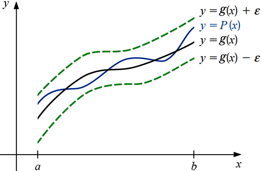
Fig. 3.1 Weierstrass Approximation Theorem. Figure is from [Burden and Faires, 2005] with minor modifications.

Interpolating Polynomial

Assume that \(n+1\) data pairs \((x_0,y_0 )\), \((x_1,y_1 )\), \((x_2 , y_2 )\), \ldots, \((x_n , y_n )\) are available in a way that the \(x_i\)s are distinct. Then, there exists a polynomial such that

(3.2)\[\begin{equation} P(x_i ) = y_i,\quad \text{for }i = 0, 1, 2, \ldots, n. \end{equation}\]

For this data, this polynomial is called the interpolating polynomial.