5.7. Techniques for Filling Missing Data in Time Series

Working with time series data containing NaN (Not a Number) values requires careful consideration to ensure accurate and meaningful analysis. Here are several effective strategies to handle NaN values in time series data [McKinney, 2022, Pandas Developers, 2023]:

5.7.1. Constant Fill

When dealing with missing values in time series data, you can use the fillna() method to fill in the gaps with a constant value or summary statistics like mean or median. This approach is useful for maintaining the overall trend and distribution of the data.

Syntax:

DataFrame.fillna(value=None, axis=None, inplace=False, limit=None, downcast=None)

Example:

import numpy as np
import pandas as pd

# Create a simple time series DataFrame with missing values
date_rng = pd.date_range(start='2023-01-01', end='2023-01-10', freq='D')
data = {'Temperature': [25.0, 24.5, np.nan, 23.0, np.nan, 22.0, 21.5, np.nan, 20.0, 19.5]}
df = pd.DataFrame(data, index=date_rng)
print("Original Data:")
display(df)

# Fill NaN values with a constant (0 in this case)
print('Filling NaN values with a constant (0):')
df_filled_constant = df.fillna(0)
display(df_filled_constant)

# Fill NaN values with the mean
_mean = df['Temperature'].mean().round(2)
print("Fill NaN values with the mean:")
df_filled_mean = df.fillna(_mean)
display(df_filled_mean)

Original Data:

	Temperature
2023-01-01	25.0
2023-01-02	24.5
2023-01-03	NaN
2023-01-04	23.0
2023-01-05	NaN
2023-01-06	22.0
2023-01-07	21.5
2023-01-08	NaN
2023-01-09	20.0
2023-01-10	19.5

Filling NaN values with a constant (0):

	Temperature
2023-01-01	25.0
2023-01-02	24.5
2023-01-03	0.0
2023-01-04	23.0
2023-01-05	0.0
2023-01-06	22.0
2023-01-07	21.5
2023-01-08	0.0
2023-01-09	20.0
2023-01-10	19.5

Fill NaN values with the mean:

	Temperature
2023-01-01	25.00
2023-01-02	24.50
2023-01-03	22.21
2023-01-04	23.00
2023-01-05	22.21
2023-01-06	22.00
2023-01-07	21.50
2023-01-08	22.21
2023-01-09	20.00
2023-01-10	19.50

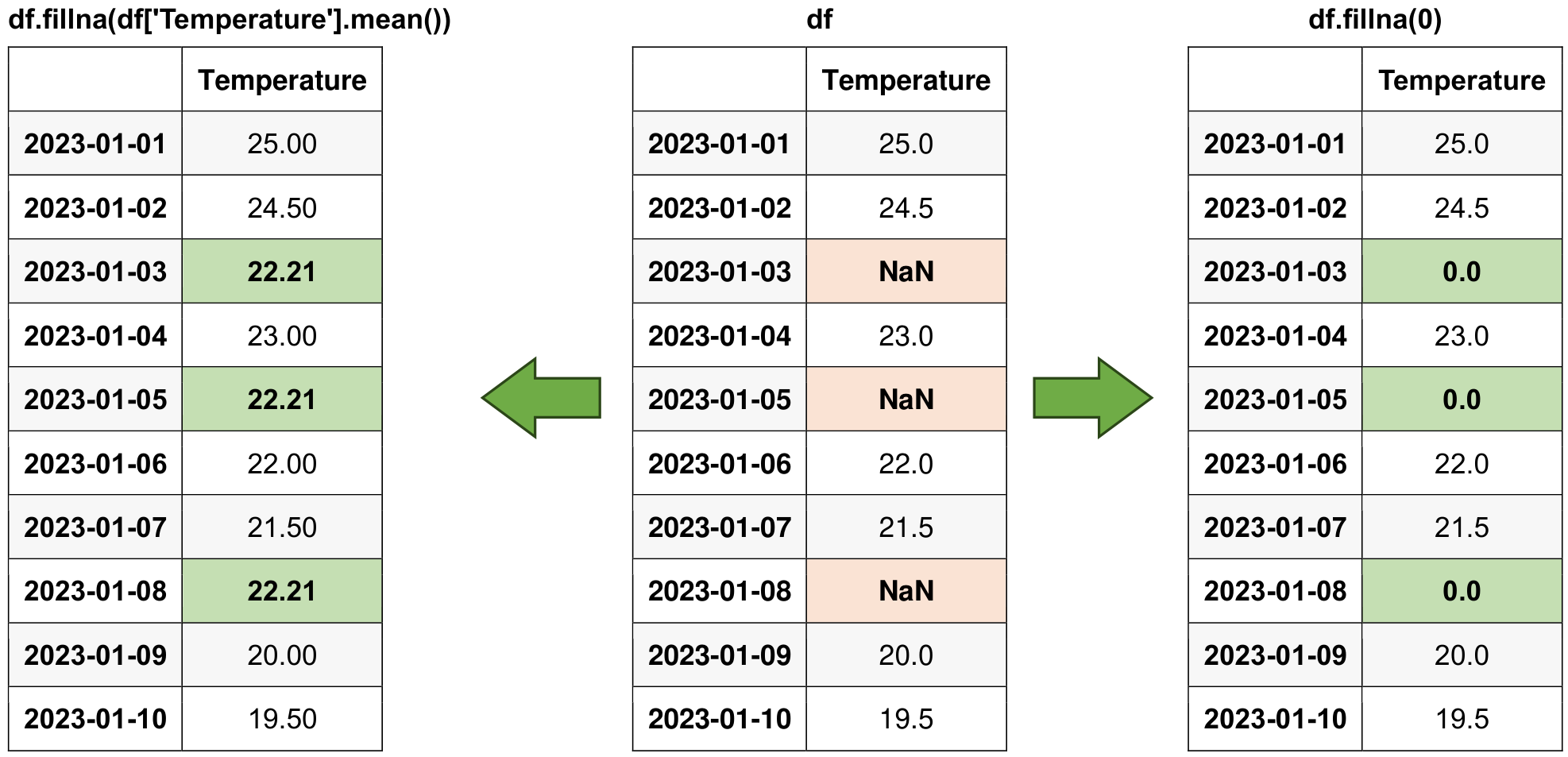
Fig. 5.12 Visual representation of the above example.

5.7.2. Forward Fill and Backward Fill

Forward fill and backward fill are methods used to handle missing values in time series data by propagating the last or next valid observation, respectively. These methods help maintain the continuity of observations in your dataset.

5.7.2.1. Forward Fill (ffill)

Forward fill (ffill) propagates the last valid observation forward to fill NaN values. This method is useful when you assume that the last known value should be carried forward.

Syntax:

DataFrame.ffill(axis=None, inplace=False, limit=None)

• axis: Specifies whether to fill missing values along rows (axis=0, default) or columns (axis=1).

• inplace: If True, modifies the original DataFrame; if False (default), returns a new DataFrame.

• limit: Limits the number of consecutive NaN values to fill.

5.7.2.2. Backward Fill (bfill)

Backward fill (bfill) propagates the next valid observation backward to fill NaN values. This method is useful when you assume that the next known value should be carried backward.

Syntax:

DataFrame.bfill(axis=None, inplace=False, limit=None)

• axis: Specifies whether to fill missing values along rows (axis=0, default) or columns (axis=1).

• inplace: If True, modifies the original DataFrame; if False (default), returns a new DataFrame.

• limit: Limits the number of consecutive NaN values to fill.

Example: An example using the same data to demonstrate both forward fill and backward fill.

import pandas as pd

# Create a simple time series DataFrame with missing values
date_rng = pd.date_range(start='2023-01-01', end='2023-01-10', freq='D')
data = {'Temperature': [25.0, 24.5, None, 23.0, None, 22.0, 21.5, None, 20.0, 19.5]}
df = pd.DataFrame(data, index=date_rng)
print("Original Data:")
display(df)

# Forward fill to propagate the last valid observation forward
df_filled_ffill = df.ffill()
print('Forward fill to propagate the last valid observation forward:')
display(df_filled_ffill)

# Backward fill to propagate the next valid observation backward
df_filled_bfill = df.bfill()
print('Backward fill to propagate the next valid observation backward:')
display(df_filled_bfill)

Original Data:

	Temperature
2023-01-01	25.0
2023-01-02	24.5
2023-01-03	NaN
2023-01-04	23.0
2023-01-05	NaN
2023-01-06	22.0
2023-01-07	21.5
2023-01-08	NaN
2023-01-09	20.0
2023-01-10	19.5

Forward fill to propagate the last valid observation forward:

	Temperature
2023-01-01	25.0
2023-01-02	24.5
2023-01-03	24.5
2023-01-04	23.0
2023-01-05	23.0
2023-01-06	22.0
2023-01-07	21.5
2023-01-08	21.5
2023-01-09	20.0
2023-01-10	19.5

Backward fill to propagate the next valid observation backward:

	Temperature
2023-01-01	25.0
2023-01-02	24.5
2023-01-03	23.0
2023-01-04	23.0
2023-01-05	22.0
2023-01-06	22.0
2023-01-07	21.5
2023-01-08	20.0
2023-01-09	20.0
2023-01-10	19.5

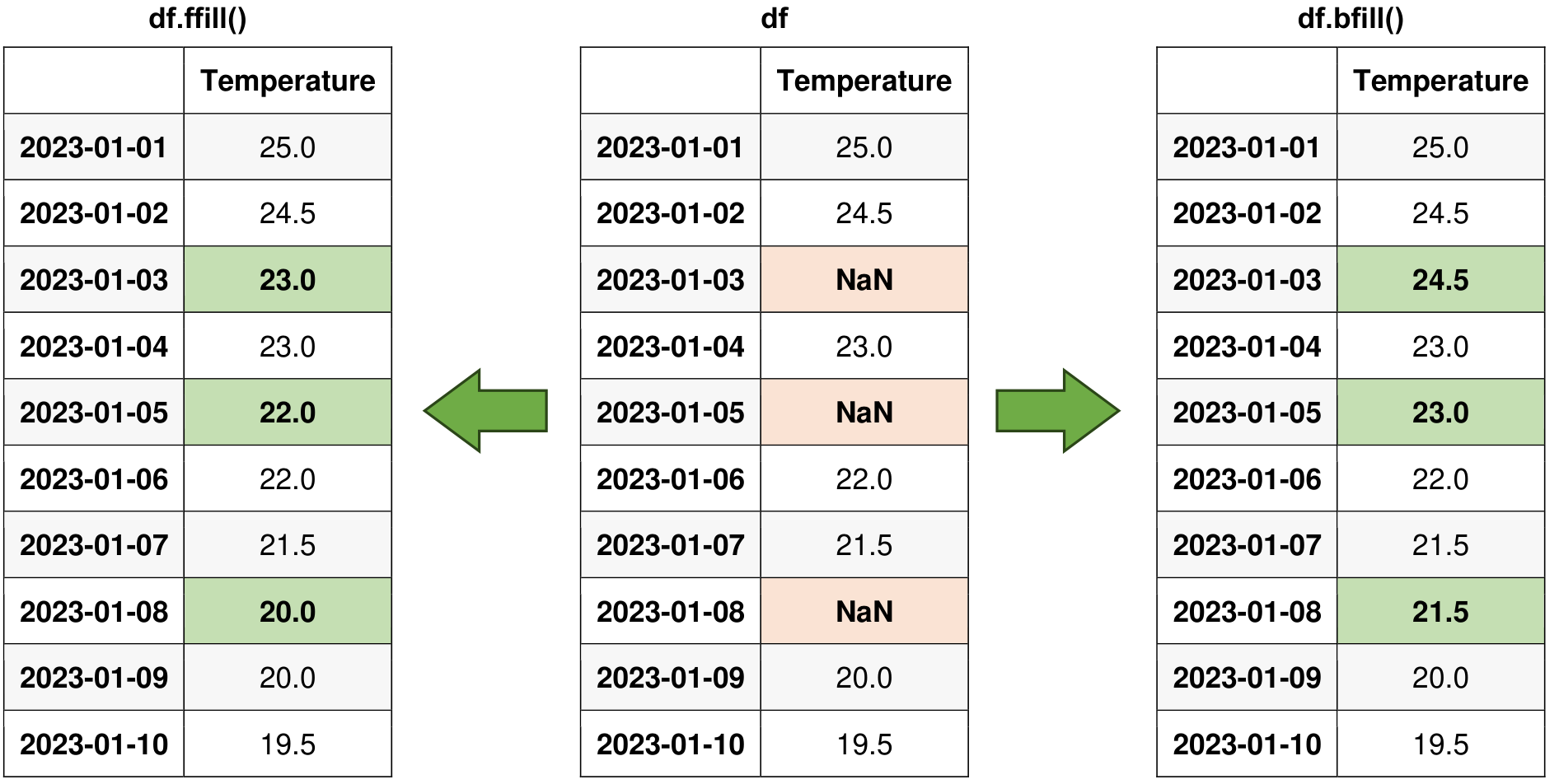
Fig. 5.13 Visual representation of the above example.

5.7.3. Filling with Interpolation

The Pandas library in Python offers the interpolate function as a versatile tool for filling missing or NaN (Not-a-Number) values within a DataFrame or Series. This function primarily employs interpolation techniques to estimate and insert values where data gaps exist [Pandas Developers, 2023].

In Pandas, interpolation works by treating the DataFrame’s index as the x-values and the column values as the y-values. This is why it’s crucial for the index to represent a logical sequence, such as time or another ordered variable, to ensure meaningful interpolation. Therefore, Pandas interpolation is not recommended when there is no logical relationship between the index and the column chosen to be interpolated.

Key Parameters:

1. method: This parameter allows you to specify the interpolation method to be used. Common methods include ‘linear,’ ‘polynomial,’ ‘spline,’ and ‘nearest,’ among others. The choice of method depends on the nature of your data and the desired interpolation behavior.

2. axis: You can specify whether the interpolation should be performed along rows (axis=0) or columns (axis=1) of the DataFrame.

3. limit: It defines the maximum number of consecutive NaN values that can be filled. This helps prevent overly aggressive data imputation.

4. limit_direction: This parameter determines whether filling should occur in a forward (‘forward’) or backward (‘backward’) direction when the ‘limit’ parameter is activated.

5. inplace: If set to True, the original DataFrame is modified in place. Otherwise, a new DataFrame with the interpolated values is returned.

• How It Works: The interpolate function uses the specified interpolation method to estimate the missing values based on the surrounding data points. For instance, with linear interpolation, missing values are estimated as points lying on a straight line between the known data points. Polynomial interpolation uses polynomial functions to approximate the missing values more flexibly. Spline interpolation constructs piecewise-defined polynomials to capture complex data patterns.

• Use Cases: Pandas’ interpolate function is particularly useful in data preprocessing, time series analysis, and data imputation tasks. It aids in maintaining the integrity of the data while ensuring a more complete dataset for downstream analysis.

You can see the function description here.

Example:

import pandas as pd
import numpy as np

# Create a simple time series DataFrame with missing values
date_rng = pd.date_range(start='2023-01-01', end='2023-01-10', freq='D')
data = {'Temperature': [25.0, 24.5, np.nan, 23.0, np.nan, 22.0, 21.5, np.nan, 20.0, 19.5]}
df = pd.DataFrame(data, index=date_rng)

# Display the original DataFrame
print("Original Data:")
display(df)

# Interpolate missing values linearly
df_interpolate = df.interpolate(method='linear')

# Display the DataFrame with missing values filled using interpolation
print("DataFrame with Missing Values Filled:")
display(df_interpolate)

Original Data:

	Temperature
2023-01-01	25.0
2023-01-02	24.5
2023-01-03	NaN
2023-01-04	23.0
2023-01-05	NaN
2023-01-06	22.0
2023-01-07	21.5
2023-01-08	NaN
2023-01-09	20.0
2023-01-10	19.5

DataFrame with Missing Values Filled:

	Temperature
2023-01-01	25.00
2023-01-02	24.50
2023-01-03	23.75
2023-01-04	23.00
2023-01-05	22.50
2023-01-06	22.00
2023-01-07	21.50
2023-01-08	20.75
2023-01-09	20.00
2023-01-10	19.50

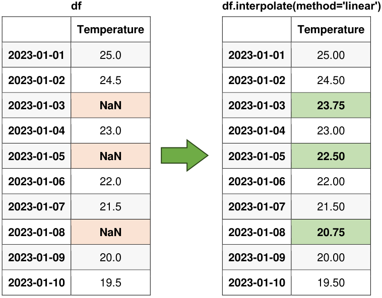
Fig. 5.14 Visual representation of the above example.

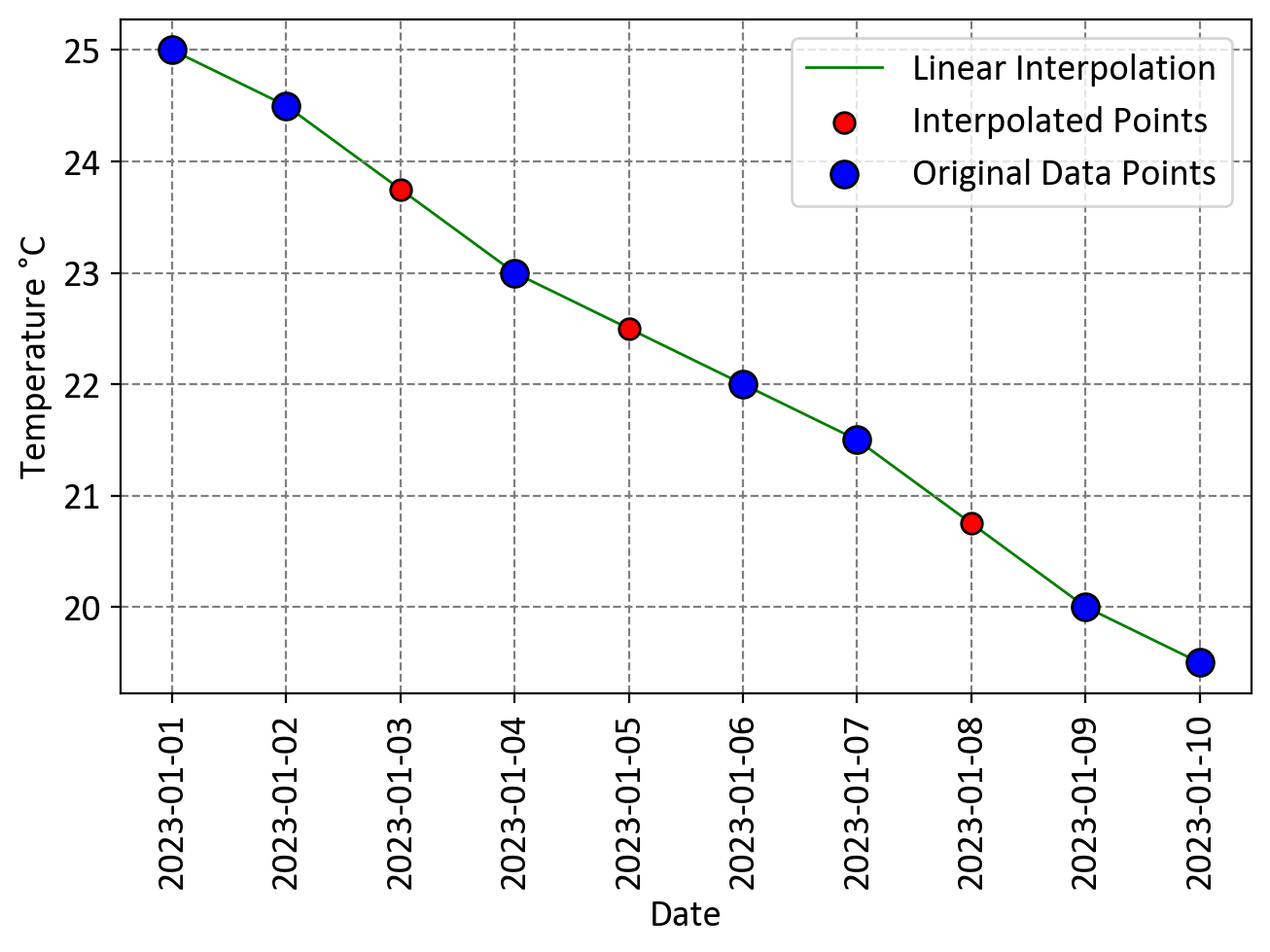
Fig. 5.15 Visual representation of pandas Linear Interpolation.

Observe that here, we can perform linear interpolation with a default numerical index.

df.reset_index(drop = True)

	Temperature
0	25.0
1	24.5
2	NaN
3	23.0
4	NaN
5	22.0
6	21.5
7	NaN
8	20.0
9	19.5

In this context, each row in the data frame is considered an individual data point, and linear interpolation is applied based on the numerical order of these data points. Let’s focus on calculating the interpolated value for the data point with the default index 2.

Assuming that the data point at default index 1 corresponds to a temperature of 24.5, and the data point at default index 3 corresponds to a temperature of 23.0, we can employ the linear interpolation formula as follows:

(5.1)\[\begin{equation} \text{Interpolated value at index 2} = 24.5 + \left( \frac{2 - 1}{3 - 1} \right) \times (23.0 - 24.5) = 23.75 \end{equation}\]

We have determined the interpolated temperature for index 2, which is 23.75. It’s worth noting that in this case, we’ve established that index 2 corresponds to the same data point as ‘2023-01-03’.

5.7.4. Dropping NaNs

When dealing with missing data, one straightforward approach is to drop rows or columns that contain NaN values using the dropna() method. This method is particularly useful when the missing values are too frequent or when estimating them is not feasible. However, it’s important to consider the impact of dropping data, as it can lead to loss of valuable information.

5.7.4.1. When to Drop NaNs

• High Frequency of Missing Values: If a significant portion of the data is missing, it might be more practical to drop those rows or columns rather than attempting to fill them.

• Unfeasible Estimation: When the missing values cannot be reliably estimated due to lack of context or insufficient data, dropping them might be the best option.

• Data Integrity: In some cases, retaining rows with missing values might compromise the integrity of the analysis. Dropping such rows ensures that the remaining data is complete and reliable.

Example: An example demonstrating how to drop rows with NaN values in a time series DataFrame:

import pandas as pd
import numpy as np

# Create a simple time series DataFrame with missing values
date_rng = pd.date_range(start='2023-01-01', end='2023-01-10', freq='D')
data = {'Temperature': [25.0, 24.5, np.nan, 23.0, np.nan, 22.0, 21.5, np.nan, 20.0, 19.5]}
df = pd.DataFrame(data, index=date_rng)

# Display the original DataFrame
print("Original Data:")
display(df)

# Drop rows with NaN values
df_dropped = df.dropna()
display(df_dropped)

Original Data:

	Temperature
2023-01-01	25.0
2023-01-02	24.5
2023-01-03	NaN
2023-01-04	23.0
2023-01-05	NaN
2023-01-06	22.0
2023-01-07	21.5
2023-01-08	NaN
2023-01-09	20.0
2023-01-10	19.5

	Temperature
2023-01-01	25.0
2023-01-02	24.5
2023-01-04	23.0
2023-01-06	22.0
2023-01-07	21.5
2023-01-09	20.0
2023-01-10	19.5

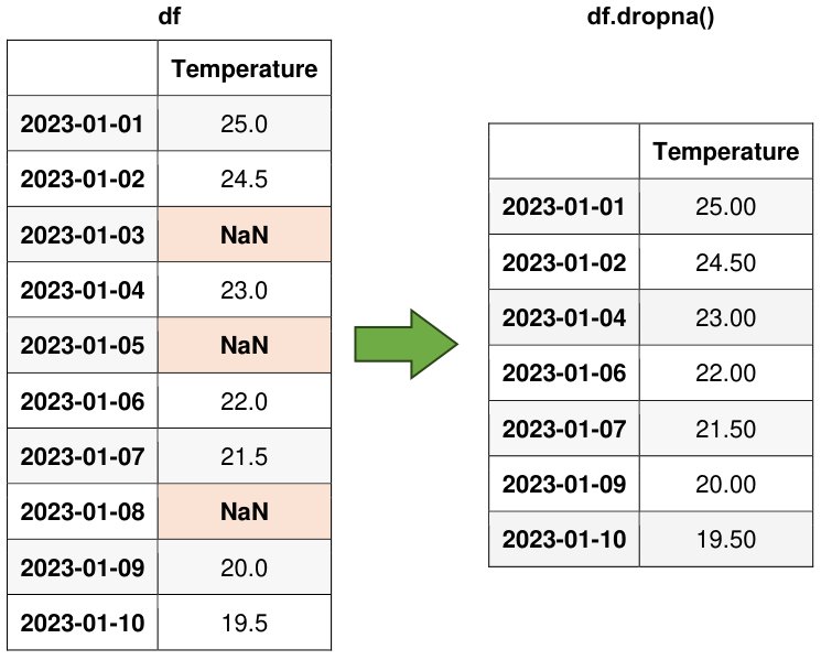
Fig. 5.16 Visual representation of the above example.

5.7.5. Imputing Missing Values through SimpleImputer

SimpleImputer is a class from the scikit-learn library in Python that provides a straightforward and flexible way to impute missing values in datasets. Imputation is the process of replacing missing values with estimated or calculated values, making the data more complete and suitable for analysis. SimpleImputer is particularly useful when we need to handle missing data in our machine learning workflow [scikit-learn Developers, 2023].

Here are the key aspects and functionalities of SimpleImputer:

1. Handling Missing Data: SimpleImputer is designed to handle missing data by replacing NaN (Not-a-Number) or other user-specified missing values with appropriate values. It can be applied to both numerical and categorical features.

2. Imputation Strategies: SimpleImputer supports various imputation strategies to replace missing values, including:

   • mean: Replaces missing values with the mean of the non-missing values in the same column (for numerical features).

   • median: Fills missing values with the median of the non-missing values in the same column (for numerical features).

   • most_frequent: Imputes missing values with the most frequent (mode) value in the same column (for categorical features).

   • constant: Replaces missing values with a user-defined constant value.

3. Usage in Machine Learning Pipelines: SimpleImputer can be integrated into scikit-learn’s machine learning pipelines, allowing you to preprocess your data and impute missing values as a part of the broader data preparation process.

4. Fit and Transform: Similar to other transformers in scikit-learn, you first fit a SimpleImputer instance on your training data using the fit method. Then, you can apply the imputation to both the training and testing datasets using the transform method.

import pandas as pd
import numpy as np
from sklearn.impute import SimpleImputer

# Create a simple time series DataFrame with missing values
date_rng = pd.date_range(start='2023-01-01', end='2023-01-10', freq='D')
data = {'Temperature': [25.0, 24.5, np.nan, 23.0, np.nan, 22.0, 21.5, np.nan, 20.0, 19.5]}
df = pd.DataFrame(data, index=date_rng)

# Display the original DataFrame
print("Original Data:")
display(df)

# Create a SimpleImputer instance to impute missing values with the mean
imputer = SimpleImputer(strategy='mean')

# Fit the imputer on the data and transform it
df_imputed = pd.DataFrame(imputer.fit_transform(df), columns=df.columns, index=df.index).round(2)

# Display the DataFrame with missing values imputed using the mean
print("DataFrame with Missing Values Imputed:")
display(df_imputed)

Original Data:

	Temperature
2023-01-01	25.0
2023-01-02	24.5
2023-01-03	NaN
2023-01-04	23.0
2023-01-05	NaN
2023-01-06	22.0
2023-01-07	21.5
2023-01-08	NaN
2023-01-09	20.0
2023-01-10	19.5

DataFrame with Missing Values Imputed:

	Temperature
2023-01-01	25.00
2023-01-02	24.50
2023-01-03	22.21
2023-01-04	23.00
2023-01-05	22.21
2023-01-06	22.00
2023-01-07	21.50
2023-01-08	22.21
2023-01-09	20.00
2023-01-10	19.50