6.4. Handling Missing Data in Pandas

Pandas strives to offer flexibility when dealing with diverse data structures. The NaN (Not a Number) value is used as the default missing value indicator due to its computational efficiency and convenience. Efficiently addressing missing data is a foundational aspect of data analysis, given that real-world datasets frequently contain incomplete or unavailable information. Pandas offers an array of methods and tools to effectively manage missing data. This article provides in-depth explanations of these techniques [McKinney, 2022, Pandas Developers, 2023].

6.4.1. Identifying Missing Data

In Pandas, the isna() and isnull() methods are used interchangeably to check for missing values within a DataFrame or Series. These methods have no functional difference; they yield identical results. Both methods generate a Boolean mask, where True indicates a missing value, and False indicates a non-missing value {cite:p}.

The choice between isna() and isnull() boils down to personal preference or coding style. Both methods exist to accommodate different user preferences. While isnull() is more commonly used, isna() is an alternative name for the same functionality. It was added for compatibility with other libraries and to enhance code readability for some users [McKinney, 2022, Pandas Developers, 2023].

Example:

import pandas as pd

data = pd.Series([1, None, 3, None, 5])

# Original Series
print("Original Series:")
print(data)

# Using isnull() to identify missing values
missing_values = data.isnull()

# displaying missing_values
print("\nIdentifying Missing Values:")
print(missing_values)

Original Series:
0    1.0
1    NaN
2    3.0
3    NaN
4    5.0
dtype: float64

Identifying Missing Values:
0    False
1     True
2    False
3     True
4    False
dtype: bool

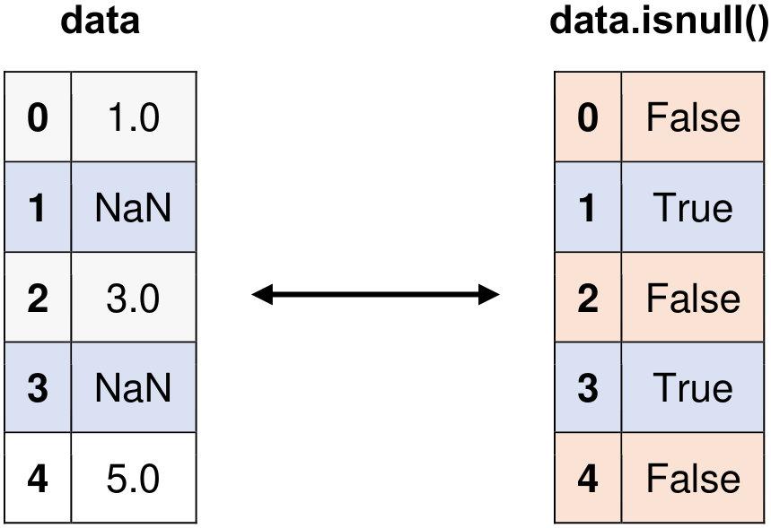
Fig. 6.8 Visual representation of the above example.

import pandas as pd

data = pd.Series([1, None, 3, None, 5])

# Original Series
print("Original Series:")
print(data)

# Using isna() to identify missing values (same as isnull())
missing_values = data.isna()

# displaying missing_values
print("\nIdentifying Missing Values with isna():")
print(missing_values)

Original Series:
0    1.0
1    NaN
2    3.0
3    NaN
4    5.0
dtype: float64

Identifying Missing Values with isna():
0    False
1     True
2    False
3     True
4    False
dtype: bool

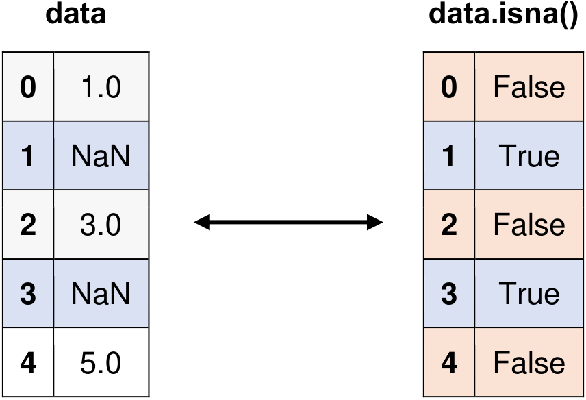
Fig. 6.9 Visual representation of the above example.

Note

Both methods, isna() and isnull(), function interchangeably, offering flexibility based on your preference or coding convention.

6.4.2. Eliminating Missing Data

In Pandas, the dropna() method is employed to eliminate missing values from a DataFrame. This method allows the removal of rows or columns that contain one or more missing values based on the specified axis. The fundamental syntax for dropna() is [McKinney, 2022, Pandas Developers, 2023]:

DataFrame.dropna(axis=0, how='any', thresh=None, subset=None, inplace=False)

Parameters:

• axis: Determines whether to drop rows with missing values (axis=0) or columns (axis=1).

• how: Specifies the conditions under which rows or columns are dropped. Possible values are 'any' (default) and 'all'. When set to 'any', any row or column containing at least one missing value will be dropped. If set to 'all', only rows or columns with all missing values will be dropped.

• thresh: An integer value setting the minimum number of non-missing values required to keep a row or column. Rows or columns with fewer non-missing values than the threshold will be dropped.

• subset: Accepts a list of column names and applies the dropna operation only to the specified columns. Other columns will be unaffected.

• inplace: When True, the original DataFrame will be modified in place, and no new DataFrame will be returned. If False (default), a new DataFrame with missing values removed will be returned, leaving the original DataFrame unchanged.

For a comprehensive reference, you can access the complete syntax description of the dropna() method here.

Example:

import pandas as pd

# Create a DataFrame with missing values
data = pd.DataFrame({'A': [1, 2, None, 4],
                     'B': [None, 6, 7, 8],
                     'C': [10, 11, None, None]})

# Drop rows containing any missing values
print('Drop rows containing any missing values:')
cleaned_data = data.dropna()
display(cleaned_data)

# Drop columns containing all missing values
print('Drop columns containing all missing values:')
cleaned_data_cols = data.dropna(axis=1, how='all')
display(cleaned_data_cols)

# Drop rows with at least 2 non-missing values
print('Drop rows with at least 2 non-missing values:')
cleaned_data_thresh = data.dropna(thresh=2)
display(cleaned_data_thresh)

Drop rows containing any missing values:

	A	B	C
1	2.0	6.0	11.0

Drop columns containing all missing values:

	A	B	C
0	1.0	NaN	10.0
1	2.0	6.0	11.0
2	NaN	7.0	NaN
3	4.0	8.0	NaN

Drop rows with at least 2 non-missing values:

	A	B	C
0	1.0	NaN	10.0
1	2.0	6.0	11.0
3	4.0	8.0	NaN

In this example, the dropna() method is used to create three distinct DataFrames with missing values removed. The first DataFrame (cleaned_data) drops rows with any missing value. The second DataFrame (cleaned_data_cols) drops columns where all values are missing. The third DataFrame (cleaned_data_thresh) drops rows with fewer than two non-missing values.

6.4.3. Filling Missing Data

6.4.3.1. Constant Fill, Forward Fill, and Backward Fill

In Pandas, the fillna() function is a versatile tool for replacing missing or NaN (Not a Number) values within a DataFrame or Series. This method is particularly useful during data preprocessing or cleaning tasks, enabling effective handling of missing data. You can tailor the way missing values are filled by using various parameters. For instance, you have the option to provide a single value, a list of values, or a dictionary to replace NaNs. Furthermore, you can employ methods like forward fill or backward fill, which carry forward the last valid value or propagate the next valid value to fill the NaNs, respectively. Additionally, you can limit the consecutive NaN values to be filled and downcast the result to a specific data type if needed. Always consider the data distribution and the analysis context to ensure the proper handling of missing data without introducing biases or inaccuracies [McKinney, 2022, Pandas Developers, 2023].

Syntax:

DataFrame.fillna(value=None, method=None, axis=None, inplace=False, limit=None, downcast=None)

The fillna() method in Pandas allows you to replace missing or NaN values within a DataFrame or Series using various options:

• The value parameter can be a single value, a list of values with the same length as the data, or a dictionary with column names as keys and values as fill values.

• You can select a specific method to fill NaNs. If no method is specified, the value will be used to fill the missing values.

• Available methods are 'fill' (or 'pad') for forward filling (propagating the last valid value forward) and 'bfill' (or 'backfill') for backward filling (propagating the next valid value backward).

• The axis parameter specifies whether to fill missing values along rows (axis=0, default) or columns (axis=1).

• When inplace=True, the original DataFrame or Series is directly modified; with inplace=False (default), a new object with filled values is returned.

• The limit parameter controls the number of consecutive NaN values filled when using forward or backward fill methods.

• The downcast parameter allows you to downcast the result to a specified data type, such as 'integer', 'signed', 'unsigned', 'float', or None (default) if possible.

You can see full description of the function here.

Example:

import pandas as pd
import warnings
warnings.simplefilter(action='ignore', category=FutureWarning)

# Creating an example DataFrame with missing values (NaN)
data = {'A': [1, 2, None, 4, 5],
        'B': [None, 10, 20, None, 50]}
df = pd.DataFrame(data)

# Displaying the original data for reference
print("Original Data:")
display(df)

# Filling NaN values with a constant (0 in this case)
print('Filling NaN values with a constant (0):')
df_filled = df.fillna(0)
display(df_filled)

# Performing forward fill to propagate previous values
print('Forward fill:')
df_ffill = df.fillna(method='ffill')
display(df_ffill)

# Performing backward fill to propagate next values
print('Backward fill:')
df_bfill = df.fillna(method='bfill')
display(df_bfill)

Original Data:

	A	B
0	1.0	NaN
1	2.0	10.0
2	NaN	20.0
3	4.0	NaN
4	5.0	50.0

Filling NaN values with a constant (0):

	A	B
0	1.0	0.0
1	2.0	10.0
2	0.0	20.0
3	4.0	0.0
4	5.0	50.0

Forward fill:

	A	B
0	1.0	NaN
1	2.0	10.0
2	2.0	20.0
3	4.0	20.0
4	5.0	50.0

Backward fill:

	A	B
0	1.0	10.0
1	2.0	10.0
2	4.0	20.0
3	4.0	50.0
4	5.0	50.0

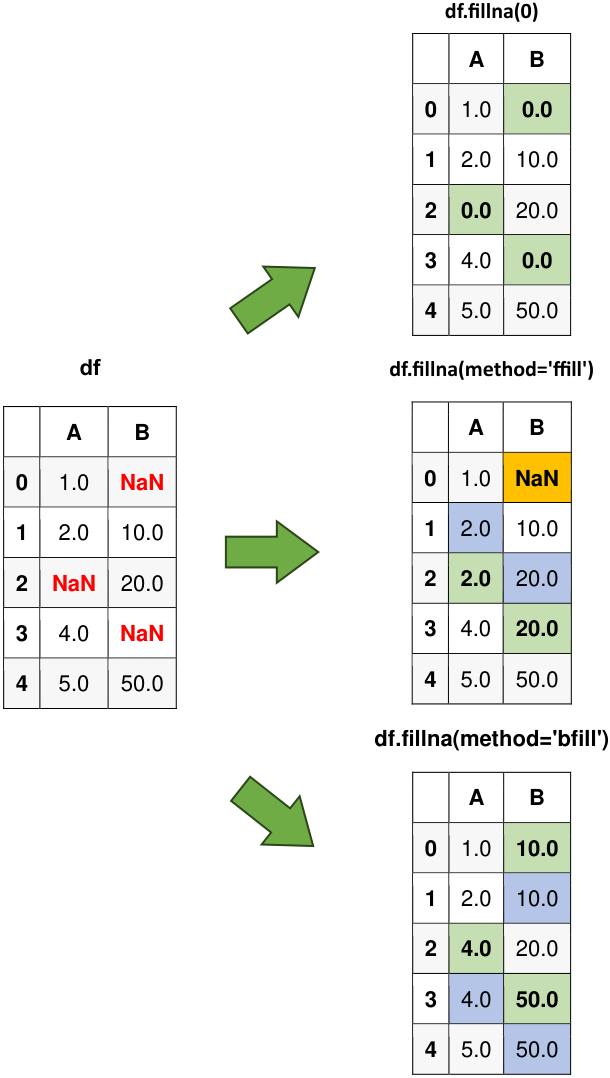
Fig. 6.10 Visual representation of the above example.

In this example, the fillna() method is used to create different DataFrames with missing values replaced. The first DataFrame (df_filled) replaces missing values with a single value. The second DataFrame (df_ffill) applies forward fill along columns. The third DataFrame (df_bfill) employs backward fill along rows.

Remark

In a recent update, the method : {‘backfill’, ‘bfill’, ‘ffill’, None} has been deprecated starting from version 2.1.0. It is recommended to use ‘ffill’ or ‘bfill’ as alternatives. Users with Pandas versions equal to or exceeding 2.1.0 will receive a future warning, although the deprecated method will continue to function for a limited number of versions beyond, such as version 2.3.

Please also see pandas.DataFrame.ffill and pandas.DataFrame.bfill.

import pandas as pd

# Creating an example DataFrame with missing values (NaN)
data = {'A': [1, 2, None, 4, 5],
        'B': [None, 10, 20, None, 50]}
df = pd.DataFrame(data)

# Displaying the original data for reference
print("Original Data:")
display(df)

# Performing forward fill to propagate previous values
print('Forward fill:')
df_ffill = df.ffill()
display(df_ffill)

# Performing backward fill to propagate next values
print('Backward fill:')
df_bfill = df.bfill()
display(df_bfill)

Original Data:

	A	B
0	1.0	NaN
1	2.0	10.0
2	NaN	20.0
3	4.0	NaN
4	5.0	50.0

Forward fill:

	A	B
0	1.0	NaN
1	2.0	10.0
2	2.0	20.0
3	4.0	20.0
4	5.0	50.0

Backward fill:

	A	B
0	1.0	10.0
1	2.0	10.0
2	4.0	20.0
3	4.0	50.0
4	5.0	50.0

6.4.3.2. Filling with Column Means or Medians

You can fill missing values with the mean or median of their respective columns. This is particularly useful when dealing with numeric data.

import pandas as pd

# Creating a DataFrame with missing values (NaN)
data = {'A': [1, 2, None, 4, 5],
        'B': [None, 10, 20, None, 50]}
df = pd.DataFrame(data)

# Displaying the original data for reference
print("Original Data:")
display(df)

# Calculating column means for NaN imputation
column_means = df.mean().round(2)

# Filling NaN values with the corresponding column means
print('Filling NaN values with column means:')
df_filled_means = df.fillna(column_means)
display(df_filled_means)

Original Data:

	A	B
0	1.0	NaN
1	2.0	10.0
2	NaN	20.0
3	4.0	NaN
4	5.0	50.0

Filling NaN values with column means:

	A	B
0	1.0	26.67
1	2.0	10.00
2	3.0	20.00
3	4.0	26.67
4	5.0	50.00

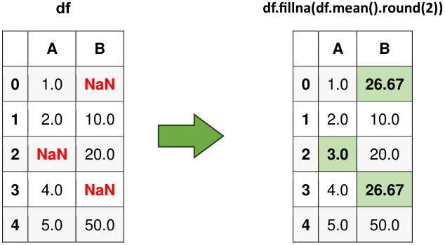
Fig. 6.11 Visual representation of the above example.

6.4.3.3. Filling with Interpolation

The Pandas library in Python offers the interpolate function as a versatile tool for filling missing or NaN (Not-a-Number) values within a DataFrame or Series. This function primarily employs interpolation techniques to estimate and insert values where data gaps exist [Pandas Developers, 2023].

Key Parameters:

1. method: This parameter allows you to specify the interpolation method to be used. Common methods include ‘linear,’ ‘polynomial,’ ‘spline,’ and ‘nearest,’ among others. The choice of method depends on the nature of your data and the desired interpolation behavior.

2. axis: You can specify whether the interpolation should be performed along rows (axis=0) or columns (axis=1) of the DataFrame.

3. limit: It defines the maximum number of consecutive NaN values that can be filled. This helps prevent overly aggressive data imputation.

4. limit_direction: This parameter determines whether filling should occur in a forward (‘forward’) or backward (‘backward’) direction when the ‘limit’ parameter is activated.

5. inplace: If set to True, the original DataFrame is modified in place. Otherwise, a new DataFrame with the interpolated values is returned.

• How It Works: The interpolate function uses the specified interpolation method to estimate the missing values based on the surrounding data points. For instance, with linear interpolation, missing values are estimated as points lying on a straight line between the known data points. Polynomial interpolation uses polynomial functions to approximate the missing values more flexibly. Spline interpolation constructs piecewise-defined polynomials to capture complex data patterns.

• Use Cases: Pandas’ interpolate function is particularly useful in data preprocessing, time series analysis, and data imputation tasks. It aids in maintaining the integrity of the data while ensuring a more complete dataset for downstream analysis.

You can see the function description here.

Example:

import pandas as pd

# Creating a DataFrame with missing values (NaN)
data = {'Value': [1, None, 3, None, 5]}
df = pd.DataFrame(data)

# Displaying the original data for reference
print("Original Data:")
display(df)

# Filling NaN values using linear interpolation
df_filled_linear = df.interpolate(method='linear')

# Displaying the DataFrame with interpolated values
print("DataFrame with interpolated values:")
display(df_filled_linear)

Original Data:

	Value
0	1.0
1	NaN
2	3.0
3	NaN
4	5.0

DataFrame with interpolated values:

	Value
0	1.0
1	2.0
2	3.0
3	4.0
4	5.0

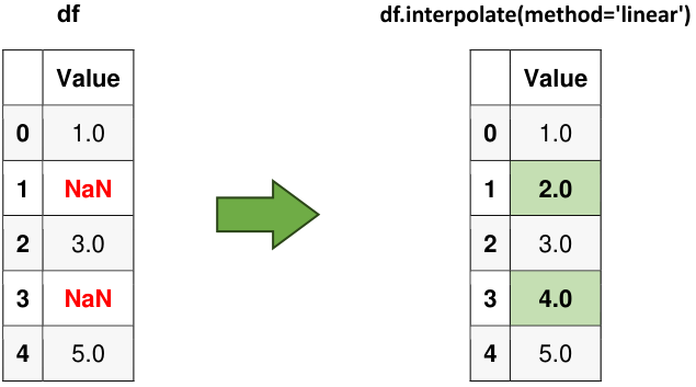
Fig. 6.12 Visual representation of the above example.

6.4.4. Working with Time Series Data

Working with time series data containing NaN (Not a Number) values requires careful consideration to ensure accurate and meaningful analysis. Here are several effective strategies to handle NaN values in time series data [McKinney, 2022, Pandas Developers, 2023]:

6.4.4.1. Constant Fill, Forward Fill or Backward Fill

As mentioned earlier, we can employ the fillna() method with either method='ffill' (for forward fill) or method='bfill' (for backward fill) to extend the last valid observation forward or the subsequent valid observation backward in order to populate the NaN values.

import numpy as np
import pandas as pd

# Create a simple time series DataFrame with missing values
date_rng = pd.date_range(start='2023-01-01', end='2023-01-10', freq='D')
data = {'Temperature': [25.0, 24.5, np.nan, 23.0, np.nan, 22.0, 21.5, np.nan, 20.0, 19.5]}
df = pd.DataFrame(data, index=date_rng)
print("Original Data:")
display(df)

# Forward fill to propagate the last valid observation forward
df_filled_ffill = df.fillna(method='ffill')
print('Forward fill to propagate the last valid observation forward:')
display(df_filled_ffill)

# Backward fill to propagate the next valid observation backward
df_filled_bfill = df.fillna(method='bfill')
print('Backward fill to propagate the next valid observation backward:')
display(df_filled_bfill)

Original Data:

	Temperature
2023-01-01	25.0
2023-01-02	24.5
2023-01-03	NaN
2023-01-04	23.0
2023-01-05	NaN
2023-01-06	22.0
2023-01-07	21.5
2023-01-08	NaN
2023-01-09	20.0
2023-01-10	19.5

Forward fill to propagate the last valid observation forward:

	Temperature
2023-01-01	25.0
2023-01-02	24.5
2023-01-03	24.5
2023-01-04	23.0
2023-01-05	23.0
2023-01-06	22.0
2023-01-07	21.5
2023-01-08	21.5
2023-01-09	20.0
2023-01-10	19.5

Backward fill to propagate the next valid observation backward:

	Temperature
2023-01-01	25.0
2023-01-02	24.5
2023-01-03	23.0
2023-01-04	23.0
2023-01-05	22.0
2023-01-06	22.0
2023-01-07	21.5
2023-01-08	20.0
2023-01-09	20.0
2023-01-10	19.5

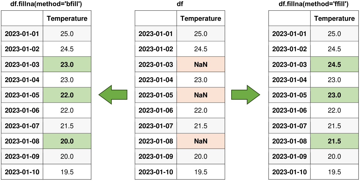
Fig. 6.13 Visual representation of the above example.

Fill NaN values with summary statistics like mean or median. We can also compute custom aggregations based on the context of our data.

import pandas as pd
import numpy as np

# Create a simple time series DataFrame with missing values
date_rng = pd.date_range(start='2023-01-01', end='2023-01-10', freq='D')
data = {'Temperature': [25.0, 24.5, np.nan, 23.0, np.nan, 22.0, 21.5, np.nan, 20.0, 19.5]}
df = pd.DataFrame(data, index=date_rng)

# Display the original DataFrame
print("Original Data:")
display(df)

# Display the DataFrame with missing values filled using interpolation
print("Fill NaN values with the mean:")
_mean = df['Temperature'].mean().round(2)
df_filled_mean = df.fillna(_mean)
display(df_filled_mean)

Original Data:

	Temperature
2023-01-01	25.0
2023-01-02	24.5
2023-01-03	NaN
2023-01-04	23.0
2023-01-05	NaN
2023-01-06	22.0
2023-01-07	21.5
2023-01-08	NaN
2023-01-09	20.0
2023-01-10	19.5

Fill NaN values with the mean:

	Temperature
2023-01-01	25.00
2023-01-02	24.50
2023-01-03	22.21
2023-01-04	23.00
2023-01-05	22.21
2023-01-06	22.00
2023-01-07	21.50
2023-01-08	22.21
2023-01-09	20.00
2023-01-10	19.50

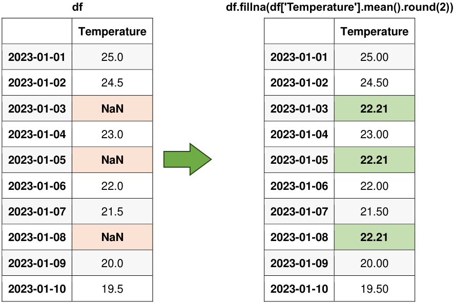
Fig. 6.14 Visual representation of the above example.

6.4.4.2. Interpolation

Similarly, as mentioned previously, Interpolation entails the estimation of missing values using available data points. The Pandas’ interpolate() method offers choices for linear, polynomial, or spline interpolation techniques. Please see this link for more details.

import pandas as pd
import numpy as np

# Create a simple time series DataFrame with missing values
date_rng = pd.date_range(start='2023-01-01', end='2023-01-10', freq='D')
data = {'Temperature': [25.0, 24.5, np.nan, 23.0, np.nan, 22.0, 21.5, np.nan, 20.0, 19.5]}
df = pd.DataFrame(data, index=date_rng)

# Display the original DataFrame
print("Original Data:")
display(df)

# Interpolate missing values linearly
df_interpolate = df.interpolate(method='linear')

# Display the DataFrame with missing values filled using interpolation
print("DataFrame with Missing Values Filled:")
display(df_interpolate)

Original Data:

	Temperature
2023-01-01	25.0
2023-01-02	24.5
2023-01-03	NaN
2023-01-04	23.0
2023-01-05	NaN
2023-01-06	22.0
2023-01-07	21.5
2023-01-08	NaN
2023-01-09	20.0
2023-01-10	19.5

DataFrame with Missing Values Filled:

	Temperature
2023-01-01	25.00
2023-01-02	24.50
2023-01-03	23.75
2023-01-04	23.00
2023-01-05	22.50
2023-01-06	22.00
2023-01-07	21.50
2023-01-08	20.75
2023-01-09	20.00
2023-01-10	19.50

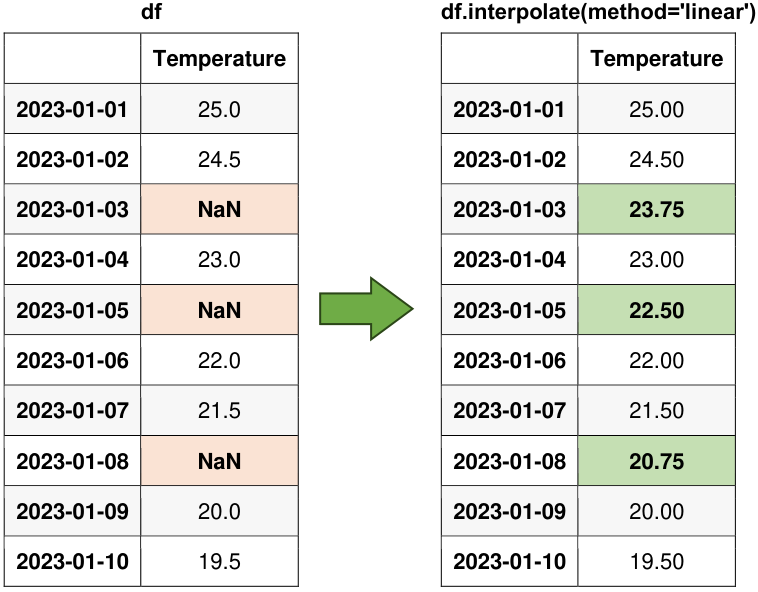
Fig. 6.15 Visual representation of the above example.

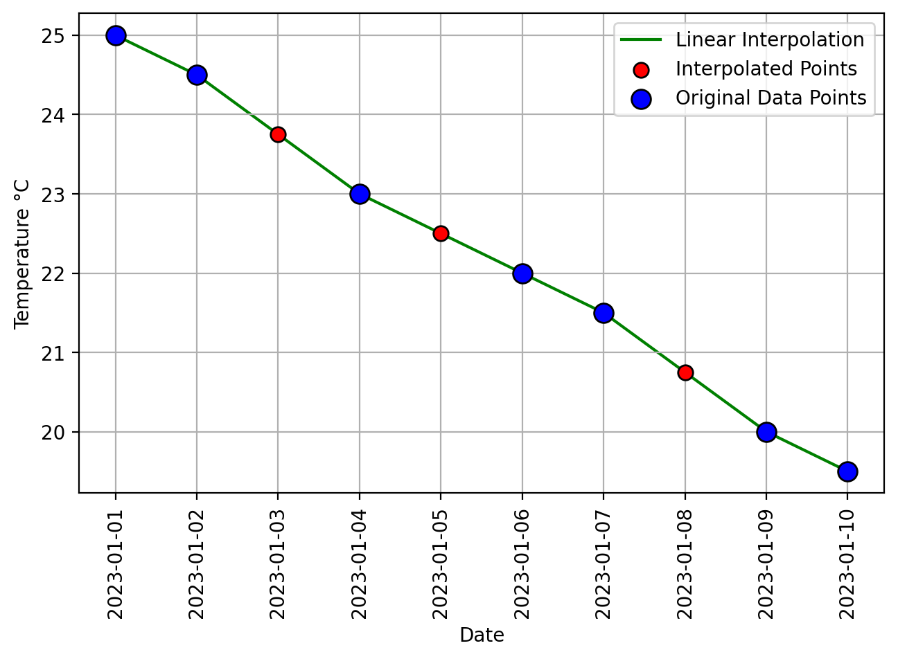
Fig. 6.16 Visual representation of pandas Linear Interpolation.

Observe that here, we can perform linear interpolation with a default numerical index.

df.reset_index(drop = True)

	Temperature
0	25.0
1	24.5
2	NaN
3	23.0
4	NaN
5	22.0
6	21.5
7	NaN
8	20.0
9	19.5

In this context, each row in the data frame is considered an individual data point, and linear interpolation is applied based on the numerical order of these data points. Let’s focus on calculating the interpolated value for the data point with the default index 2.

Assuming that the data point at default index 1 corresponds to a temperature of 24.5, and the data point at default index 3 corresponds to a temperature of 23.0, we can employ the linear interpolation formula as follows:

(6.1)\[\begin{equation} \text{Interpolated value at index 2} = 24.5 + \left( \frac{2 - 1}{3 - 1} \right) \times (23.0 - 24.5) = 23.75 \end{equation}\]

We have determined the interpolated temperature for index 2, which is 23.75. It’s worth noting that in this case, we’ve established that index 2 corresponds to the same data point as ‘2023-01-03’.

6.4.4.3. Dropping NaNs

Consider dropping rows with NaN values using the dropna() method if the missing values are too frequent or unfeasible to estimate.

import pandas as pd
import numpy as np

# Create a simple time series DataFrame with missing values
date_rng = pd.date_range(start='2023-01-01', end='2023-01-10', freq='D')
data = {'Temperature': [25.0, 24.5, np.nan, 23.0, np.nan, 22.0, 21.5, np.nan, 20.0, 19.5]}
df = pd.DataFrame(data, index=date_rng)

# Display the original DataFrame
print("Original Data:")
display(df)

# Drop rows with NaN values
df_dropped = df.dropna()
display(df_dropped)

Original Data:

	Temperature
2023-01-01	25.0
2023-01-02	24.5
2023-01-03	NaN
2023-01-04	23.0
2023-01-05	NaN
2023-01-06	22.0
2023-01-07	21.5
2023-01-08	NaN
2023-01-09	20.0
2023-01-10	19.5

	Temperature
2023-01-01	25.0
2023-01-02	24.5
2023-01-04	23.0
2023-01-06	22.0
2023-01-07	21.5
2023-01-09	20.0
2023-01-10	19.5

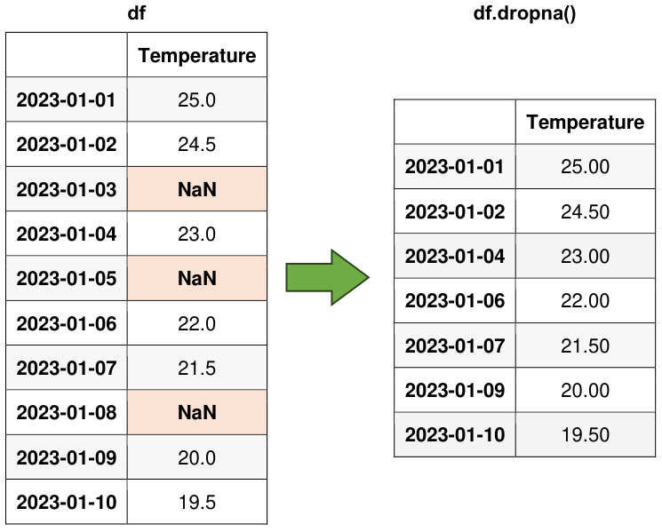
Fig. 6.17 Visual representation of the above example.

6.4.4.4. Imputing Missing Values through SimpleImputer

SimpleImputer is a class from the scikit-learn library in Python that provides a straightforward and flexible way to impute missing values in datasets. Imputation is the process of replacing missing values with estimated or calculated values, making the data more complete and suitable for analysis. SimpleImputer is particularly useful when we need to handle missing data in our machine learning workflow [scikit-learn Developers, 2023].

Here are the key aspects and functionalities of SimpleImputer:

1. Handling Missing Data: SimpleImputer is designed to handle missing data by replacing NaN (Not-a-Number) or other user-specified missing values with appropriate values. It can be applied to both numerical and categorical features.

2. Imputation Strategies: SimpleImputer supports various imputation strategies to replace missing values, including:

   • mean: Replaces missing values with the mean of the non-missing values in the same column (for numerical features).

   • median: Fills missing values with the median of the non-missing values in the same column (for numerical features).

   • most_frequent: Imputes missing values with the most frequent (mode) value in the same column (for categorical features).

   • constant: Replaces missing values with a user-defined constant value.

3. Usage in Machine Learning Pipelines: SimpleImputer can be integrated into scikit-learn’s machine learning pipelines, allowing you to preprocess your data and impute missing values as a part of the broader data preparation process.

4. Fit and Transform: Similar to other transformers in scikit-learn, you first fit a SimpleImputer instance on your training data using the fit method. Then, you can apply the imputation to both the training and testing datasets using the transform method.

import pandas as pd
import numpy as np
from sklearn.impute import SimpleImputer

# Create a simple time series DataFrame with missing values
date_rng = pd.date_range(start='2023-01-01', end='2023-01-10', freq='D')
data = {'Temperature': [25.0, 24.5, np.nan, 23.0, np.nan, 22.0, 21.5, np.nan, 20.0, 19.5]}
df = pd.DataFrame(data, index=date_rng)

# Display the original DataFrame
print("Original Data:")
display(df)

# Create a SimpleImputer instance to impute missing values with the mean
imputer = SimpleImputer(strategy='mean')

# Fit the imputer on the data and transform it
df_imputed = pd.DataFrame(imputer.fit_transform(df), columns=df.columns, index=df.index).round(2)

# Display the DataFrame with missing values imputed using the mean
print("DataFrame with Missing Values Imputed:")
display(df_imputed)

Original Data:

	Temperature
2023-01-01	25.0
2023-01-02	24.5
2023-01-03	NaN
2023-01-04	23.0
2023-01-05	NaN
2023-01-06	22.0
2023-01-07	21.5
2023-01-08	NaN
2023-01-09	20.0
2023-01-10	19.5

DataFrame with Missing Values Imputed:

	Temperature
2023-01-01	25.00
2023-01-02	24.50
2023-01-03	22.21
2023-01-04	23.00
2023-01-05	22.21
2023-01-06	22.00
2023-01-07	21.50
2023-01-08	22.21
2023-01-09	20.00
2023-01-10	19.50

6.4.5. Strategies for Handling Missing Categorical Data in Pandas

Managing missing categorical data in pandas is crucial for preserving data quality and conducting meaningful analyses. To address this issue, we can consider the following effective strategies:

6.4.5.1. Leaving Missing Values as NaN

In some scenarios, it is advisable to maintain categorical values as NaNs (Not a Number) when they are missing. This approach can be appropriate when the absence of data conveys valuable information or carries significance.

By retaining missing categorical values as NaNs, we ensure that the missingness itself is treated as a distinct category, allowing our analysis to capture the potential significance of missing data. This approach is particularly valuable when the missingness pattern has meaning in our dataset, such as in surveys where “prefer not to answer” is a valid response [Mccaffrey, 2020].

6.4.5.2. Impute Missing Categorical Values with the Most Frequent Category

To handle missing categorical values effectively, a practical approach is to impute them with the most frequently occurring category within the respective column. This strategy ensures that missing data is replaced with a category that maintains the overall distribution of the data, minimizing potential bias in your analysis [Pandas Developers, 2023].

Example:

import pandas as pd

# Create a DataFrame with missing categorical values
data = {'Category': ['A', 'B', 'C', None, 'A', None, 'B']}
df = pd.DataFrame(data)

# Display the original DataFrame
print("Original DataFrame:")
display(df)

# Impute missing values with the most frequent category
most_frequent_category = df['Category'].mode()[0]
df['Category'].fillna(most_frequent_category, inplace=True)

# Display the DataFrame with missing values filled using the most frequent category
print("DataFrame with Missing Values Filled:")
display(df)

Original DataFrame:

	Category
0	A
1	B
2	C
3	None
4	A
5	None
6	B

DataFrame with Missing Values Filled:

	Category
0	A
1	B
2	C
3	A
4	A
5	A
6	B

In this example, the missing categorical values are replaced with the most frequent category, ensuring that the distribution of categories remains representative of the original data.

6.4.5.3. Imputing Missing Categorical Values with a Specific Category

When dealing with missing categorical values, it is often beneficial to replace them with a designated category that signifies the absence of data or a special category chosen for this purpose. This approach ensures that the missingness is clearly indicated in our dataset and prevents any ambiguity when interpreting the results of our analysis [Pandas Developers, 2023].

Example:

import pandas as pd

# Create a DataFrame with missing categorical values
data = {'Category': ['A', 'B', None, 'C', 'B']}
df = pd.DataFrame(data)

# Display the original DataFrame
print("Original DataFrame:")
display(df)

# Fill missing values with a specific category, e.g., 'Unknown'
specific_category = 'Unknown'
df['Category'].fillna(specific_category, inplace=True)

# Display the DataFrame with missing values filled using the specific category
print("DataFrame with Missing Values Filled:")
display(df)

Original DataFrame:

	Category
0	A
1	B
2	None
3	C
4	B

DataFrame with Missing Values Filled:

	Category
0	A
1	B
2	Unknown
3	C
4	B

In this example, missing categorical values are replaced with the designated category ‘Unknown,’ making it explicit that these values were missing originally.

6.4.5.4. Predictive Models for Imputing Missing Categorical Values

In our data analysis process, we have the option to employ machine learning models to predict missing categorical values based on the information available in the dataset.

6.4.5.5. Eliminating Rows with Missing Categorical Data

In situations where the presence of missing categorical values is limited, and their removal does not substantially impact our analysis, we can opt to remove the rows containing these missing data points.

6.4.6. Advantages and Disadvantages of Imputing Missing Data

In the context of data analysis, imputing missing data, whether in Pandas or any other data analysis tool, is a common practice. However, it comes with its set of advantages and disadvantages [Data, 2016, Little and Rubin, 2019]. Here, we outline the key considerations:

Advantages of Imputing Missing Data:

1. Preserving Data Integrity: Imputing missing data allows us to retain more data points in our analysis, thereby preserving the overall integrity of our dataset.

2. Avoiding Bias: The removal of rows with missing data can introduce bias if the missingness is not entirely random. Imputation helps mitigate bias by replacing missing values with plausible estimates.

3. Statistical Power: Imputation enhances the statistical power of our analysis since we have more data to work with, potentially leading to more robust results.

4. Compatibility with Algorithms: Many machine learning and statistical algorithms require complete datasets. Imputing missing data renders our dataset compatible with a wider range of modeling techniques.

5. Enhancing Visualizations: Imputed data can improve the quality of visualizations and exploratory data analysis by providing a more comprehensive view of our dataset.

Disadvantages of Imputing Missing Data:

1. Potential Bias: Imputing missing data introduces the potential for bias if the chosen imputation method is not suitable for the underlying data distribution or the mechanism causing the missingness.

2. Loss of Information: Imputing missing data may result in the loss of information, especially if the imputed values do not accurately represent the missing data.

3. Inaccurate Estimates: Imputed values may not precisely reflect the true values of the missing data, particularly when the missingness is due to unique or unobservable factors.

4. Increased Variability: Imputed data can increase the variability in our dataset, potentially affecting the stability of our analyses.

5. Complexity: The selection of the appropriate imputation method and the handling of missing data can be complex, especially in datasets with multiple variables and diverse missing data patterns.