Spatial Resolution

1.4. Spatial Resolution#

Spatial resolution refers to the size of one pixel on the ground. A higher spatial resolution indicates more detail and a smaller area covered by each pixel [Earth Science Data Systems, 2019].

Consider a patchwork quilt covering the ground, where each square of the quilt represents a pixel in an image. The spatial resolution is the size of these squares. Smaller squares (pixels) mean that the quilt (image) can show finer patterns and details. For instance, a high spatial resolution of 30 centimeters per pixel allows us to distinguish between objects like cars and trees, while a lower resolution might only show larger features like buildings or fields.

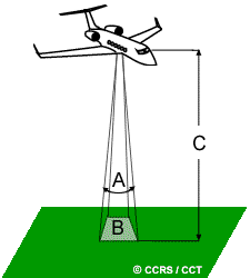
Fig. 1.11 illustrates the concept of spatial resolution in remote sensing [Natural Resources Canada, 2007]:

A - Instantaneous Field of View (IFOV): This is the angular cone of visibility of the sensor, defining the area of the Earth’s surface visible from the sensor at any given moment. A smaller IFOV results in finer spatial resolution.
B - Area on the Earth’s Surface (Spatial Resolution): This shaded area represents the part of the Earth’s surface that falls within the IFOV, indicating the ground area the sensor can capture in an image at one time.
C - Distance Between the Ground and Sensor: This is the altitude of the sensor above the Earth’s surface. The size of the resolution cell, which determines the maximum spatial resolution, is calculated by multiplying the IFOV by this distance.

../_images/fieldview.png — Fig. 1.11 The spatial resolution of the sensor is illustrated by the smallest detectable feature on the ground, represented by point A within the sensor’s field of view. Image Credit: [Natural Resources Canada, 2007]. Link to the image.#

1.4.1. Field of View (FOV) and Instantaneous Field of View (IFOV)#

1.4.1.1. Field of View (FOV)#

The Field of View (FOV) is the angle of vision that the entire focal plane array (FPA) matrix covers from the objective’s second node [Pencheva et al., 2006].

(1.2)#\[FOV = \dfrac{a}{f} = \dfrac{A}{s}\]

where:

$a$ = dimension of the FPA matrix
$f$ = focal length of the objective
$A$ = dimension of the object
$s$ = distance to the object plane

Note

Objective: The lens or optical system that focuses light onto the FPA detector.
Object: The target or scene being observed or imaged.
FPA Detector: The focal plane array, a sensor matrix that captures the image formed by the objective.

1.4.1.2. Instantaneous Field of View (IFOV)#

The Instantaneous Field of View (IFOV) is the angle of vision of a single pixel of the photo-receiving matrix from the objective’s second node [Pencheva et al., 2006].

(1.3)#\[IFOV = \dfrac{\delta a}{f} = \dfrac{\delta A}{s}\]

where:

$\delta a$ = dimension of one pixel of the FPA matrix
$\delta A$ = projection size of one pixel on the object plane

These equations help determine the resolution and field of vision for infrared optical systems.

Moreover, Fig. 1.12 illustrates the Field of View (FOV) and Instantaneous Field of View (IFOV) for an optical system:

Field of View (FOV): This is the angle of vision of the entire focal plane array (FPA) matrix from the objective’s second node [Pencheva et al., 2006]. It is calculated as $FOV = a / f = A / s$, where $a$ is the dimension of the FPA, $f$ is the focal length, $A$ is the image dimension, and $s$ is the distance to the object plane.
Instantaneous Field of View (IFOV): This is the angle of vision of a single pixel of the photo-receiving matrix from the objective’s second node [Pencheva et al., 2006]. It is calculated as $IFOV = \delta a / f = \delta A / s$, where $\delta a$ is the dimension of one pixel.

These parameters help determine the resolution and quality of the infrared imaging system.

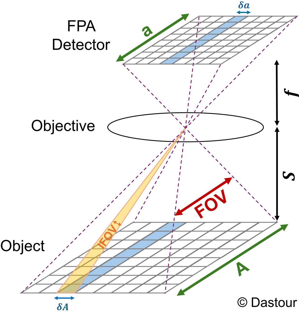
../_images/field_of_view.jpg — Fig. 1.12 The spatial resolution of the sensor is illustrated by the smallest detectable feature on the ground, represented by point A within the sensor’s field of view. Image reproduced based on the idea presented in [Pencheva *et al.*, 2006].#

Example 1.2

Given Parameters

Dimension of the FPA matrix ($a$): 20 mm
Focal length of the objective ($f$): 50 mm
Distance to the object plane ($s$): 1000 mm
Dimension of one pixel of the FPA matrix ($\delta a$): 0.02 mm

Field of View (FOV): Using the formula (1.2), and substituting the given values:

\[\begin{equation*} FOV = \dfrac{20 \, \text{mm}}{50 \, \text{mm}} = 0.4 \end{equation*}\]

This means the FOV is 0.4 radians.

Instantaneous Field of View (IFOV): Using the formula (1.3), and substituting the given values:

\[\begin{equation*} IFOV = \dfrac{0.02 \, \text{mm}}{50 \, \text{mm}} = 0.0004 \end{equation*}\]

This means the IFOV is 0.0004 radians.

Interpretation:

The FOV of the entire FPA matrix is 0.4 radians, which indicates the angle of vision covered by the entire sensor array.
The IFOV of a single pixel is 0.0004 radians, which indicates the angle of vision covered by a single pixel in the sensor array.

1.4.2. Importance of Spatial Resolution in Remote Sensing#

Spatial resolution measures the smallest feature a sensor can detect. The IFOV and the sensor’s altitude work together to define the resolution cell, the smallest area on the ground that can be resolved. If a feature is larger than the resolution cell, it can be detected; if it is smaller, it may not be distinguishable unless it has a dominant reflectance that allows for sub-pixel detection. This concept is crucial for understanding the capabilities and limitations of different remote sensing technologies.

Spatial resolution is critical in satellite imagery, determining how much detail is visible. For example, the Moderate Resolution Imaging Spectroradiometer (MODIS) instruments on the Terra and Aqua satellites have bands with different resolutions:

1 km Resolution Bands: These bands are suited for observing large-scale environmental changes. Each pixel represents a 1 km² area on the ground, offering a broader view but with less detail.
250 m and 500 m Resolution Bands: These higher-resolution bands capture smaller areas of 250 m² and 500 m² per pixel, respectively. They are ideal for detailed monitoring and mapping of smaller regions.

The difference in detail is evident when comparing images with varying resolutions:

A 30 m/pixel resolution image shows fine details with little to no pixelation.
At 100 m/pixel, the image is less detailed, and objects become harder to distinguish.
At 300 m/pixel, the image is quite pixelated, suitable only for identifying large features.

Example 1.3

Fig. 1.13 provides a visual comparison of the city of Calgary using satellite imagery from the USGS Landsat 8 Level 2, Collection 2, Tier 1 dataset. Each panel represents the city at a different spatial resolution, demonstrating how the level of detail changes with varying pixel sizes. The panels show the city at four different resolutions:

30 m/pixel: The highest resolution, where individual features such as roads, buildings, and vegetation patches are more discernible.
100 m/pixel: A moderate resolution where some details are still visible, but finer features start to blur.
300 m/pixel: Lower resolution, where urban features become less distinct.

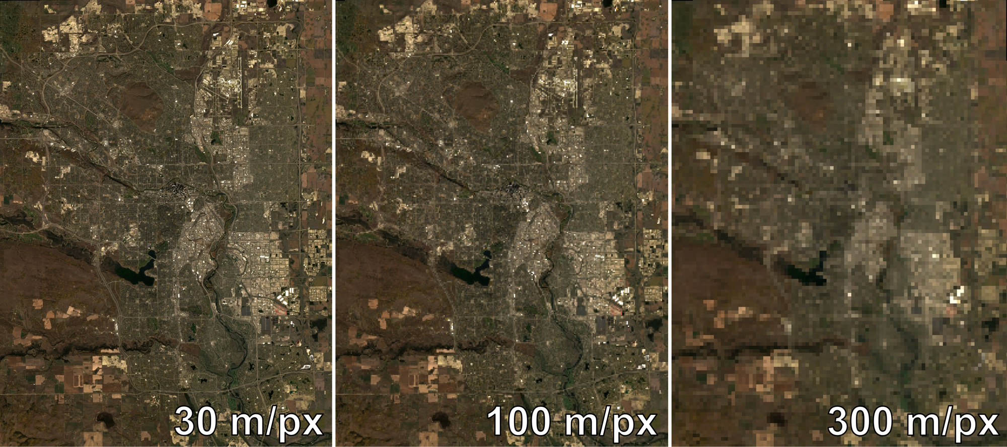
../_images/Landsat432_Calgary.jpg — Fig. 1.13 Panels showing the city of Calgary using the Red, Green, and Blue bands from USGS Landsat 8 Level 2, Collection 2, Tier 1. The images are displayed at different spatial resolutions: 30 m/pixel, 100 m/pixel, and 300 m/pixel. Image processed by H. Dastour using Google Earth Engine. Note: JPG format for web display and the image processed by H. Dastour using Google Earth Engine.#

This figure effectively illustrates the impact of spatial resolution on satellite imagery and highlights the importance of selecting appropriate resolutions for different applications. Higher resolutions provide more detailed information, which is crucial for applications like urban planning, environmental monitoring, and geographical analysis.

1.4.3. What Spatial Resolution Should We Use?#

Fig. 1.14 provides a visual guide to understanding spatial resolution in the context of Earth observation. It explains that spatial resolution is the area represented by a single pixel in an image, with examples ranging from coarse to fine resolutions [Earth Science Data Systems, 2019]:

Lowest/Coarse (110 km / 1 degree): Suitable for global observations, this resolution provides a broad overview of Earth’s features but lacks detail.
Continental (30 km / 0.25 degrees): This resolution is appropriate for studying large-scale phenomena across continents.
National (10 km / 0.09 degrees): With more detail, this resolution is good for country-wide research, capturing features like large cities or natural parks.
Regional (1 km): This fine resolution allows for detailed studies of smaller areas, such as neighborhoods or specific ecosystems.

The infographic emphasizes the importance of choosing the right spatial resolution for different scales of research, from global to regional studies.

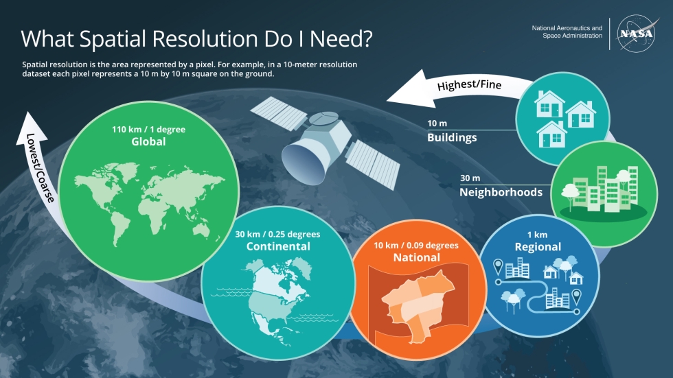
../_images/Spatial-Resolution-Basics.jpeg — Fig. 1.14 A range of spatial resolutions available for common NASA sensor products, tailored for diverse research needs from local to global extents. Link to Image.#

1.4.4. Swaths: The Breadth of Earth Observation#

In remote sensing, “swath” refers to the segment of the Earth’s surface captured by a sensor aboard a satellite or aircraft in a single flyover. It’s comparable to the panoramic view from an airplane window—the swath is the visible strip of land below, representing the sensor’s field of vision during one orbit around the Earth [Natural Resources Canada, 2007].

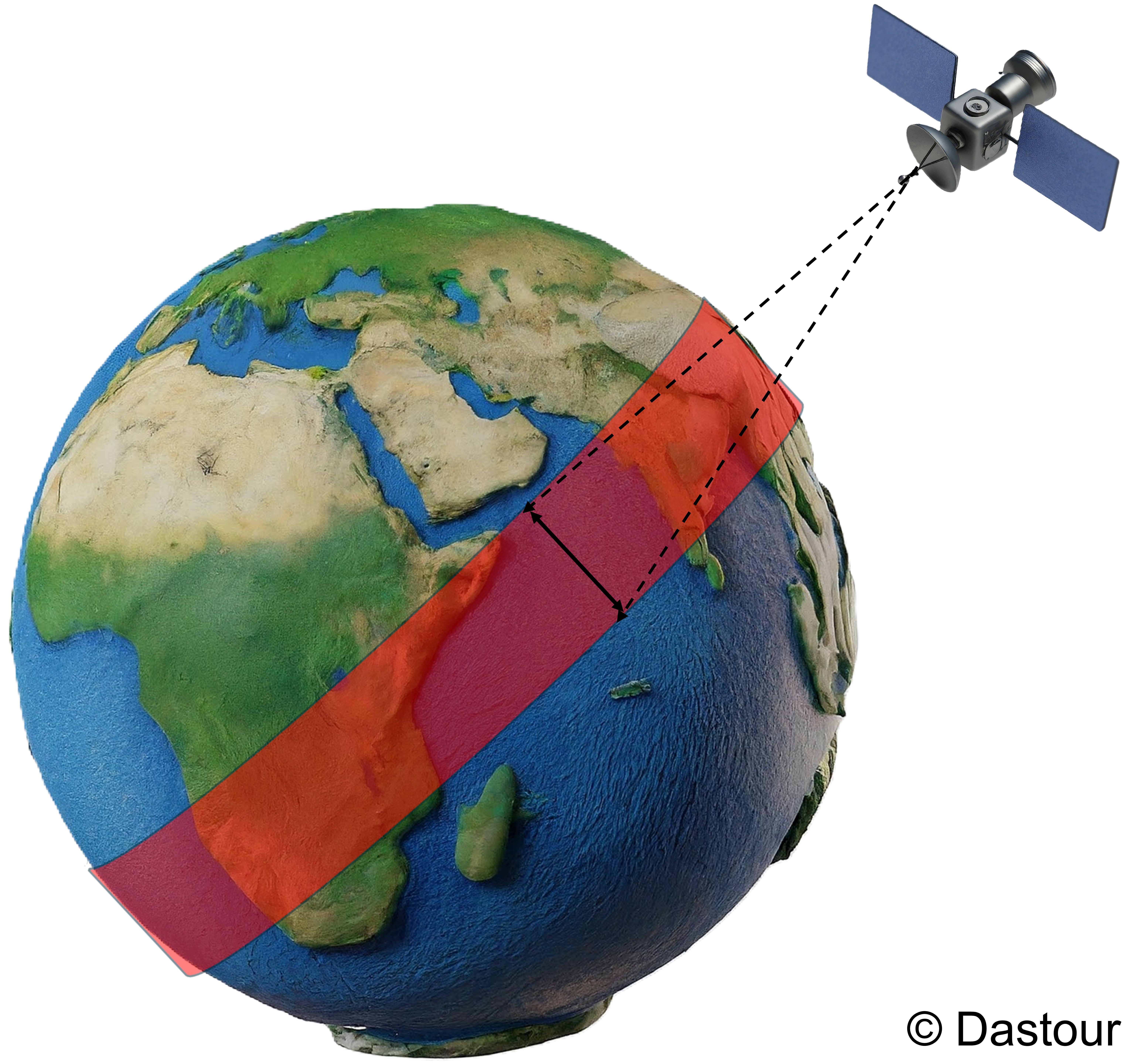
../_images/bandwidth.jpg — Fig. 1.15 A satellite orbiting the Earth, the swath would be the area on the Earth’s surface that the satellite is able to image during a single pass.#

The swath’s width is determined by two key factors:

Sensor’s Field of View (FOV): The angular range within which the sensor can observe and collect data.
Satellite’s Altitude: The height at which the satellite orbits the Earth.

Example 1.4 (High vs. Low Swath Width)

Wide FOV and Low Earth Orbit (LEO): A sensor with a wide FOV on an LEO satellite will have a larger swath, covering more ground with each pass.
Narrow FOV and High Earth Orbit (HEO): A sensor with a narrow FOV on a HEO satellite will have a smaller swath, covering less ground with each pass.

The closer a satellite is to the Earth’s surface, the narrower the area it can image. Conversely, satellites at higher altitudes can cover wider areas.

Fig. 1.16 illustrates the calculation of swath width $W$ for a satellite sensor’s field of view using the following formula:

(1.4)#\[ W = 2H \tan(\theta) \]

where:

$H$ is the altitude of the satellite above the Earth’s surface.
$\theta$ is the half-angle of the sensor’s field of view.

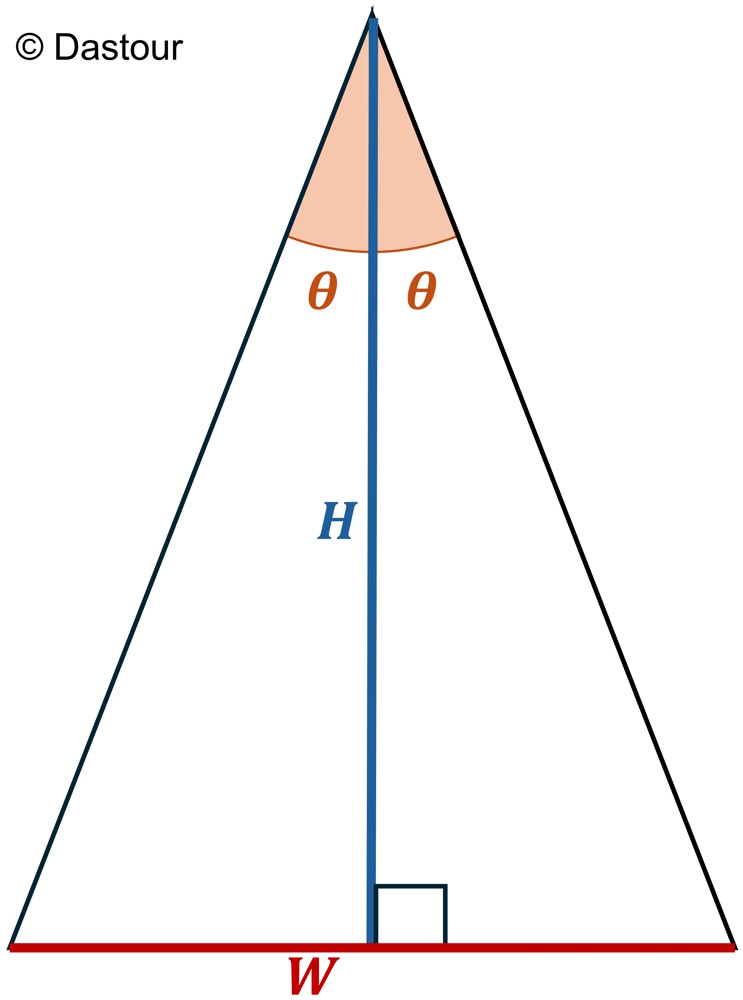
../_images/sw_fig.jpg — Fig. 1.16 Geometric illustration showing how swath width ($W$) is calculated from satellite altitude ($H$) and sensor half-angle field of view ($\theta$).#

Explanation:

Altitude ($H$): This is the height of the satellite above the Earth’s surface. For example, if a satellite is at an altitude of 500 km, $H = 500 $ km.
Field of View Angle ($2\theta$): The total viewing angle of the sensor. For instance, if the sensor has a full field of view angle of 136 degrees, the half-angle $\theta$ would be 68 degrees.

Example 1.5

Suppose a satellite is at an altitude of 833 km and the sensor’s half-angle of the field of view ($\theta) is 60°.

Using the formula (1.4)

Where:

$W$ is the swath width
$H$ is the satellite altitude (833 km)
$θ$ is the half-angle of the field of view (60°)

Calculation: $W = 2 \times 833 \times \tan(60°) = 1666 \times 1.73 ≈ 2885.60$ km

Thus, for a satellite at 833 km altitude with a sensor half-angle of 60°, the swath width would be approximately 2886 km.

Additional Considerations:

Geometrical Properties: The swath width can vary based on the geometrical properties of the satellite’s orbit and the sensor’s design.
Resolution: The swath width also affects the spatial resolution of the images captured. A wider swath generally means lower spatial resolution and vice versa.

This formula and explanation provide a basic understanding of how to calculate the swath width of a satellite based on its altitude and sensor characteristics.

1.4.5. Importance of Swath Width#

Swath size is crucial in remote sensing as it affects:

The extent of the Earth’s surface that can be imaged.
The frequency at which a specific location is revisited, which is tied to the concept of temporal resolution.

A larger swath enables satellites to map extensive areas more quickly, which is vital in the design and application of remote sensing technologies. Understanding swath dimensions is key to planning thorough and regular imaging of particular areas.

Fig. 1.17 compares the orbital swath coverage of two different Earth observation instruments:

MODIS (Moderate Resolution Imaging Spectroradiometer): Illustrated by blue boxes, MODIS boasts a considerably wider imaging swath, enabling it to cover a larger portion of the Earth’s surface per pass and provide global coverage every 1-2 days.
OLI (Operational Land Imager) aboard Landsat 8: Displayed as boxes with red dots, the OLI has a narrower swath than MODIS, leading to a longer interval, approximately 16 days, to achieve global coverage.

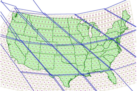
../_images/landsatmodis.png — Fig. 1.17 Orbital swath of MODIS (blue boxes) versus the orbital swath of the OLI aboard Landsat 8 (boxes with red dots). Due to its much wider imaging swath, MODIS provides global coverage every 1-2 days versus 16 days for the OLI. Red dots indicate the center point of each Landsat tile. Image Credit: NASA Applied Remote Sensing Training (ARSET). Link to Image#

Fig. 1.17 effectively demonstrates the impact of swath width on the temporal resolution of satellite imagery. A wider swath, like that of MODIS, enables more frequent revisits to the same location on Earth, which is beneficial for monitoring changes over time. In contrast, the narrower swath of OLI results in less frequent coverage but can provide higher spatial resolution imagery.

For example, MODIS is ideal for tracking large-scale environmental changes such as deforestation and urban expansion due to its frequent coverage. Meanwhile, OLI is suitable for detailed analysis of smaller areas with high spatial resolution, such as monitoring crop health or urban infrastructure.

Spatial Resolution

Contents

1.4. Spatial Resolution#

1.4.1. Field of View (FOV) and Instantaneous Field of View (IFOV)#

1.4.1.1. Field of View (FOV)#

1.4.1.2. Instantaneous Field of View (IFOV)#

1.4.2. Importance of Spatial Resolution in Remote Sensing#

1.4.3. What Spatial Resolution Should We Use?#

1.4.4. Swaths: The Breadth of Earth Observation#

1.4.5. Importance of Swath Width#