12.2. Fundamentals of Neural Networks#
12.2.1. Neurons and Their Role in Computational Modeling#
Neurons are like the building blocks of artificial neural networks (ANNs), and they’re inspired by how our brains work. Just like how our own brain cells process and share information, artificial neurons do a similar job. When it comes to ANNs, neurons act as the workers that take in data and turn it into something useful [Aggarwal, 2023, Mehlig, 2021, Ye, 2022]. Think of these neurons as tiny processors. They take the information given to them, adjust its importance, do some calculations, and then give out a result. This process happens layer by layer, and it’s really good at finding patterns in data. This is why neural networks are great at things like recognizing pictures and understanding language. They’re like the brains behind some really smart computer programs.
12.2.1.1. Key Elements of an Artificial Neuron:#
Inputs: Neurons receive data from the preceding layer or directly from the input dataset. Each piece of input data represents various attributes, features, or facets of the information under scrutiny.
Weights: Think of weights as significance labels for the input data. These weights determine the importance of each piece of information in shaping the neuron’s output. During the learning process, these weights are adjusted to optimize the neuron’s predictive abilities.
Bias: A bias serves as an additional factor that enhances the neuron’s adaptability and flexibility. Visualize it as an adjustable knob fine-tuning the neuron’s behavior, enabling it to better comprehend intricate relationships within the data.
Summation: All the weighted inputs and the bias are aggregated, much like assembling puzzle pieces to reveal a larger picture. This summation, executed in a specific manner, illustrates how all the individual input components interrelate.
Activation Function: The aggregated result from the previous step undergoes an activation function. This function determines the neuron’s response pattern, akin to its “disposition.” The disposition can range from positive to negative or fall somewhere in between, playing a crucial role in processing diverse data patterns.
Output: The activation function yields the neuron’s “decision” or interpretation of the data. It articulates, “I believe this is the meaning of the data.” This decision can then propagate to other neurons, progressively constructing a deeper comprehension of the information. Alternatively, if it belongs to the final layer, it can constitute the network’s ultimate conclusion or prediction.
In essence, an artificial neuron operates as a miniature decision-maker, ingesting information, evaluating its importance, and delivering its perspective on the matter. When numerous neurons collaborate, they exhibit remarkable capabilities, such as pattern recognition and deciphering intricate data structures [Aggarwal, 2023, Mehlig, 2021, Ye, 2022].
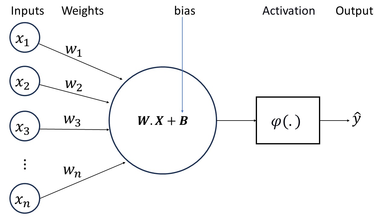
Fig. 12.1 The main usage of the Activation Function is to convert the aggregated and weighted input from a node into an output value that can be propagated to the next hidden layer or used as an output.#
Example: A linear transformation stands as a pivotal building block, forming the basis upon which more complex architectures are constructed. At its core, a linear transformation takes input data and performs a weighted combination of its features, ultimately yielding an output. This process is encapsulated by the mathematical equation \(z = W.X + B\), where \(z\) signifies the resulting output [Bengio, 2009, Goodfellow et al., 2016, LeCun et al., 2015].
Components of a Linear Transformation:
Output (\(z\)): The output \(z\) represents the result of the linear transformation. It encapsulates the synthesized information that arises from the combination of input features according to learned weights and biases. While this transformation might seem simplistic, its elegance lies in its foundation—a direct linear relationship between inputs and outputs [Bengio, 2009, Goodfellow et al., 2016, LeCun et al., 2015].
Weight Matrix (\(W\)) The weight matrix \(W\) is the crux of the linear transformation. This matrix encompasses the learned weights assigned to each feature in the input data. In essence, it determines the influence that each feature wields in the process of generating the output. The arrangement of these weights in the matrix permits a holistic view of the interplay between input features and their corresponding importance [Bengio, 2009, Goodfellow et al., 2016, LeCun et al., 2015].
Input Matrix (\(X\)): The input matrix \(X\) forms the bedrock of the transformation. Comprising rows of input samples and columns of distinct features, \(X\) encapsulates the raw information that the model processes. Each column of the matrix corresponds to a specific feature, and each row corresponds to an individual sample. This representation allows the linear transformation to operate simultaneously on multiple samples, making it a vectorized and efficient computation [Bengio, 2009, Goodfellow et al., 2016, LeCun et al., 2015].
Bias Matrix (\(B\)): While the weight matrix captures the interactions between input features, the bias matrix \(B\) introduces an additional degree of freedom. It is a vector that is added element-wise to the weighted sum of features before producing the final output. This term permits the model to account for inherent offsets or baseline values that are not directly captured by the weighted features alone [Bengio, 2009, Goodfellow et al., 2016, LeCun et al., 2015].
12.2.1.2. Computation and Learning in Neural Networks#
The inner workings of an artificial neuron closely emulate the information processing mechanisms of biological neurons. Yet, the true potential of artificial neurons is unlocked when they are orchestrated into layered configurations, interconnected to establish a neural network. Within this network, neurons cooperate in a concerted effort to acquire the ability to convert raw input data into coherent and meaningful representations. This collective learning process equips the network to make predictions and execute various tasks founded upon the acquired knowledge of patterns [Aggarwal, 2023, Mehlig, 2021, Ye, 2022].
12.2.2. Activation Functions#
As we journey from simple linear models to the complex landscapes of deep learning, activation functions step forward as vital agents of transformation. Their essence lies in imparting neural networks with the power to capture non-linear phenomena, opening pathways for representing intricate data relationships. By transcending the boundaries of linear operations, activation functions unlock the network’s potential to tackle tasks that involve subtle patterns and complex interactions.
12.2.2.1. The Role of Activation Functions#
Deep learning activation functions are mathematical functions that are applied to the output of a layer of a neural network. They determine how the output of the layer is transformed into the input for the next layer, or the final prediction of the model. Activation functions are essential for deep learning because they introduce non-linearity into the network, which allows it to learn complex patterns from data [Bengio, 2009, Goodfellow et al., 2016, LeCun et al., 2015].
Fig. 12.2 The main usage of the Activation Function is to convert the aggregated and weighted input from a node into an output value that can be propagated to the next hidden layer or used as an output.#
There are many types of activation functions that have different properties and effects on the network performance. Some of the most common activation functions are:
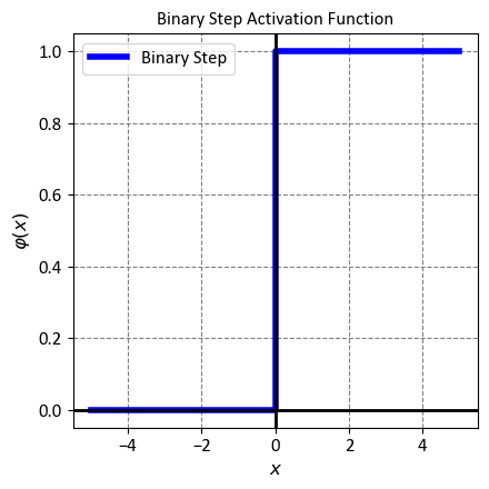
12.2.2.2. Binary Step function#
The Binary Step function is a simple activation function used in binary classification tasks, where the output of a neuron or a model needs to be binary, often representing classes like 0 and 1. Mathematically, the Binary Step function is defined as follows:
Here, \(x\) is the input to the function. The Binary Step function returns 0 if the input is less than 0, and it returns 1 if the input is greater than or equal to 0. It essentially provides a threshold-based output where any positive input is mapped to the value 1 and any negative input is mapped to the value 0.
Show code cell source
import numpy as np
import matplotlib.pyplot as plt
plt.style.use('../mystyle.mplstyle')

# Define the Binary Step function
def binary_step(x):
    return np.where(x >= 0, 1, 0)

# Generate x values
x = np.linspace(-5, 5, 100)

# Apply the Binary Step function to x values
y = binary_step(x)

# Create the plot using subplots
fig, ax = plt.subplots(figsize=(4.5, 4.5))
_ = ax.step(x, y, label='Binary Step', color='blue', linewidth=4, where='mid')
_ = ax.axhline(0, color='black', linewidth=2, linestyle='-')
_ = ax.axvline(0, color='black', linewidth=2, linestyle='-')
_ = ax.set(xlabel=r'$x$', ylabel= r'$\varphi(x)$',
           title='Binary Step Activation Function')
_ = ax.legend(fontsize = 12)
_ = ax.grid(True)
plt.tight_layout()
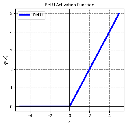
12.2.2.3. ReLU (Rectified Linear Unit)#
The Rectified Linear Unit, or ReLU for short, is a simple but powerful activation function that is widely used in deep learning models. It is defined as a piecewise linear function that outputs zero for negative inputs and the input itself for positive inputs. Mathematically, the ReLU function is expressed as:
ReLU has several advantages over other activation functions, such as sigmoid or tanh. First, it is easy to compute and implement, which reduces the computational cost and complexity of the model. Second, it helps to mitigate the vanishing gradient problem, which occurs when the gradients of the activation function become too small to effectively update the weights of the model. This problem can hamper the learning process and lead to poor performance. ReLU avoids this issue by having a constant gradient of one for positive inputs, which ensures a steady flow of error signals during backpropagation. Third, it introduces non-linearity and sparsity into the model, which can enhance the expressive power and generalization ability of the model. ReLU can create sparse representations by setting some of the outputs to zero, which can reduce the correlation and redundancy among the features [Dubey et al., 2022, Goodfellow et al., 2016, He et al., 2015].
However, ReLU is not without drawbacks. One of the main challenges of using ReLU is the dying ReLU problem, which occurs when some of the neurons become inactive and stop producing any output. This can happen when the inputs to the ReLU function are negative for a long period of time, which causes the gradients to be zero and prevents any weight updates. As a result, the neurons can get stuck in a state where they always output zero, regardless of the input. This can reduce the effective capacity of the model and lead to poor performance. Several variants of ReLU have been proposed to address this problem, such as Leaky ReLU, Parametric ReLU, and Exponential Linear Unit (ELU) [Clevert et al., 2015, He et al., 2015, Maas et al., 2013].
Show code cell source
import numpy as np
import matplotlib.pyplot as plt

# Define the ReLU function
def relu(x):
    return np.maximum(0, x)

# Generate x values
x = np.linspace(-5, 5, 100)

# Apply the ReLU function to x values
y = relu(x)

# Create the plot using subplots
fig, ax = plt.subplots(figsize=(4.5, 4.5))
_ = ax.plot(x, y, label='ReLU', color='blue', linewidth=4)
_ = ax.axhline(0, color='black', linewidth=2, linestyle='-')
_ = ax.axvline(0, color='black', linewidth=2, linestyle='-')
_ = ax.set(xlabel=r'$x$', ylabel= r'$\varphi(x)$',
           title='ReLU Activation Function')
_ = ax.legend(fontsize = 12)
_ = ax.grid(True)
plt.tight_layout()
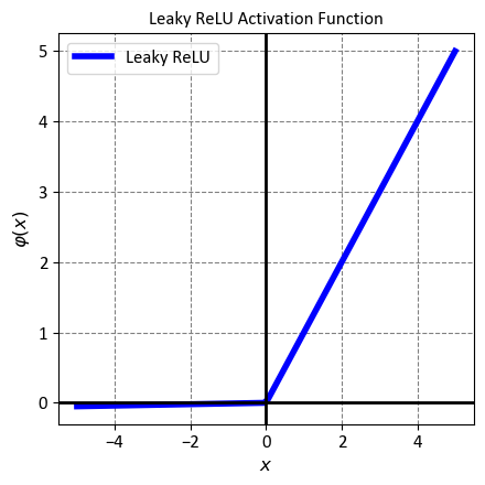
12.2.2.4. Leaky ReLU#
Leaky ReLU is a variant of the Rectified Linear Unit (ReLU) activation function that aims to overcome the drawbacks of the standard ReLU function. Unlike ReLU, which outputs zero for negative inputs, Leaky ReLU allows a small, non-zero output for negative inputs. This can prevent the neurons from becoming inactive and improve the performance of the neural network. Mathematically, Leaky ReLU is defined as:
where \(x\) is the input to the function, and \(\alpha\) is a small positive constant (typically 0.01). The function can be interpreted as follows:
For positive inputs, Leaky ReLU behaves like the identity function, meaning it preserves the input value without any change.
For negative inputs, Leaky ReLU scales the input by a factor of \(\alpha\), resulting in a linear function with a slope of \(\alpha\). This ensures that the output is not zero and the gradient can flow through the function.
Leaky ReLU has several benefits over ReLU, such as [Maas et al., 2013, Xu et al., 2015]:
It avoids the dying ReLU problem, where some neurons can stop learning due to zero gradients. By allowing a small output for negative inputs, Leaky ReLU ensures that the neurons remain active and responsive to the input variations.
It introduces a slight asymmetry and non-linearity into the function, which can enhance the expressive power and generalization ability of the neural network. Leaky ReLU can create sparse and diverse representations by setting some of the outputs to a small value, which can reduce the correlation and redundancy among the features.
It is easy to implement and computationally efficient, which makes it suitable for large-scale and complex models.
Show code cell source
import numpy as np
import matplotlib.pyplot as plt

# Define the Leaky ReLU function
def leaky_relu(x, alpha=0.01):
    return np.maximum(alpha * x, x)

# Generate x values
x = np.linspace(-5, 5, 100)

# Apply the Leaky ReLU function to x values
y = leaky_relu(x)

# Create the plot using subplots
fig, ax = plt.subplots(figsize=(4.5, 4.5))
_ = ax.plot(x, y, label='Leaky ReLU', color='blue', linewidth=4)
_ = ax.axhline(0, color='black', linewidth=2, linestyle='-')
_ = ax.axvline(0, color='black', linewidth=2, linestyle='-')
_ = ax.set(xlabel=r'$x$', ylabel= r'$\varphi(x)$',
           title='Leaky ReLU Activation Function')
_ = ax.legend(fontsize = 12)
_ = ax.grid(True)
plt.tight_layout()
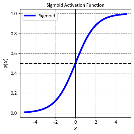
12.2.2.5. Sigmoid Function#
The Sigmoid function is a classic activation function that is widely used in machine learning and deep learning models. It is a smooth and continuous function that maps any real-valued input to a value between 0 and 1. This property makes it suitable for tasks that require output probabilities, such as binary classification or logistic regression. Mathematically, the Sigmoid function is expressed as:
where \(x\) is the input to the function, and \(e\) is the base of the natural logarithm. The function can be interpreted as follows:
For large positive inputs, the Sigmoid function approaches 1, meaning it assigns a high probability to the positive class.
For large negative inputs, the Sigmoid function approaches 0, meaning it assigns a low probability to the positive class.
For inputs close to zero, the Sigmoid function outputs a value close to 0.5, meaning it assigns an equal probability to both classes.
The Sigmoid function has several advantages, such as [Goodfellow et al., 2016]:
It is easy to implement and understand, which makes it a popular choice for beginners and practitioners.
It is differentiable and has a simple derivative, which facilitates the gradient-based optimization methods.
It introduces non-linearity and saturation into the model, which can enhance the expressive power and robustness of the model. Sigmoid can create bounded and smooth representations by compressing the input range to a fixed interval, which can reduce the sensitivity and variance of the output.
However, the Sigmoid function also has some drawbacks, such as [Glorot et al., 2011, Krizhevsky et al., 2017, Nair and Hinton, 2010]:
It suffers from the vanishing gradient problem, which occurs when the gradients of the activation function become too small to effectively update the weights of the model. This problem can hamper the learning process and lead to poor performance. Sigmoid is prone to this issue because it has a very flat region at both ends of the curve, where the gradient is almost zero.
It is not zero-centered, meaning it does not have a mean of zero. This can cause a shift in the distribution of the inputs to the next layer, which can affect the learning dynamics and convergence of the model. Sigmoid can create unbalanced and biased representations by shifting the input mean to a positive value, which can increase the correlation and redundancy among the features.
It is computationally expensive, meaning it requires more time and resources to calculate and evaluate. This can limit the scalability and efficiency of the model. Sigmoid involves an exponential operation, which is more costly than a linear or piecewise linear operation.
Show code cell source
import numpy as np
import matplotlib.pyplot as plt

# Define the Sigmoid function
def sigmoid(x):
    return 1 / (1 + np.exp(-x))

# Generate x values
x = np.linspace(-5, 5, 100)

# Apply the Sigmoid function to x values
y = sigmoid(x)

# Create the plot using subplots
fig, ax = plt.subplots(figsize=(4.5, 4.5))
_ = ax.plot(x, y, label='Sigmoid', color='blue', linewidth=4)
_ = ax.axhline(0.5, color='black', linewidth=2, linestyle='--')
_ = ax.axvline(0, color='black', linewidth=2, linestyle='-')
_ = ax.set(xlabel=r'$x$', ylabel= r'$\varphi(x)$',
           title='Sigmoid Activation Function')
_ = ax.legend(fontsize = 12)
_ = ax.grid(True)
plt.tight_layout()
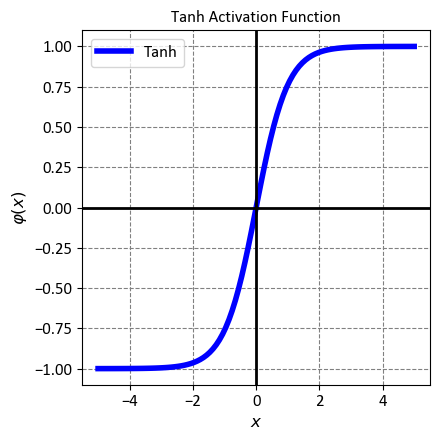
12.2.2.6. Tanh (Hyperbolic Tangent)#
The Hyperbolic Tangent, or Tanh for short, is a smooth and continuous activation function that is widely used in machine learning and deep learning models. It is a scaled and shifted version of the Sigmoid function, meaning it maps any real-valued input to a value between -1 and 1. This property makes it suitable for tasks that require output values to be centered around zero, such as regression or sentiment analysis. Mathematically, the Tanh function is expressed as:
where \(x\) is the input to the function, and \(e\) is the base of the natural logarithm. The function can be interpreted as follows:
For large positive inputs, the Tanh function approaches 1, meaning it assigns a high positive value to the input.
For large negative inputs, the Tanh function approaches -1, meaning it assigns a high negative value to the input.
For inputs close to zero, the Tanh function outputs a value close to zero, meaning it assigns a neutral value to the input.
The Tanh function has several advantages over the Sigmoid function, such as [Goodfellow et al., 2016, LeCun et al., 2015]:
It is zero-centered, meaning it has a mean of zero. This can prevent a shift in the distribution of the inputs to the next layer, which can improve the learning dynamics and convergence of the model. Tanh can create balanced and symmetrical representations by mapping the input range to a symmetric interval, which can reduce the correlation and redundancy among the features.
It is steeper than the Sigmoid function, meaning it has a larger gradient for a given input. This can speed up the learning process and lead to better performance. Tanh can create more distinct and diverse representations by separating the input values more clearly, which can increase the sensitivity and variance of the output.
However, the Tanh function also has some drawbacks, such as [Bengio, 2009, Goodfellow et al., 2016]:
It still suffers from the vanishing gradient problem, although to a lesser extent than the Sigmoid function. This occurs when the gradients of the activation function become too small to effectively update the weights of the model. This problem can hamper the learning process and lead to poor performance. Tanh is prone to this issue because it still has a very flat region at both ends of the curve, where the gradient is almost zero.
It is not optimal for tasks that require output probabilities, such as binary classification or logistic regression. This is because it outputs values between -1 and 1, which are not interpretable as probabilities. Tanh can create ambiguous and misleading representations by assigning negative values to some of the inputs, which can confuse the model and the user.
Show code cell source
import numpy as np
import matplotlib.pyplot as plt

# Define the Hyperbolic Tangent (Tanh) function
# Generate x values
x = np.linspace(-5, 5, 100)

# Apply the Tanh function to x values
y = np.tanh(x)

# Create the plot using subplots
fig, ax = plt.subplots(figsize=(4.5, 4.5))
_ = ax.plot(x, y, label='Tanh', color='blue', linewidth=4)
_ = ax.axhline(0, color='black', linewidth=2, linestyle='-')
_ = ax.axvline(0, color='black', linewidth=2, linestyle='-')
_ = ax.set(xlabel=r'$x$', ylabel= r'$\varphi(x)$',
           title='Tanh Activation Function')
_ = ax.legend(fontsize = 12)
_ = ax.grid(True)
plt.tight_layout()
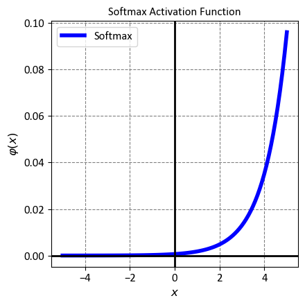
12.2.2.7. Softmax#
The Softmax function is a popular activation function that is often used in the output layer of a neural network. It is a generalization of the logistic function, meaning it can handle multiple classes instead of just two. It is also known as the normalized exponential function, because it normalizes the input values by using the exponential function. Mathematically, the Softmax function is defined as:
where \(p_i\) is the output probability for the \(i\)-th class, \(x_i\) is the input score or logit for the \(i\)-th class, \(e\) is the base of the natural logarithm, and \(n\) is the total number of classes. The function can be interpreted as follows:
For each class, the Softmax function computes the exponential of the input score, which can amplify the difference between the scores and make the largest score more dominant.
For each class, the Softmax function divides the exponential of the input score by the sum of the exponentials of all the input scores, which can ensure that the output probabilities sum up to one and form a valid probability distribution.
The Softmax function outputs a vector of probabilities, where each element represents the likelihood of the input belonging to a certain class. The class with the highest probability is the predicted class for the input.
The Softmax function has several advantages, such as [Bishop, 2016, Goodfellow et al., 2016]:
It is differentiable and has a simple derivative, which facilitates the gradient-based optimization methods.
It is compatible with the cross-entropy loss function, which is a common choice for measuring the discrepancy between the predicted probabilities and the true labels.
It is invariant to scaling, meaning it does not change the output probabilities if the input scores are multiplied by a constant factor. This can prevent numerical issues and improve the stability of the model.
Show code cell source
import numpy as np
import matplotlib.pyplot as plt

# Define the Softmax function
def softmax(x):
    exp_x = np.exp(x - np.max(x))  # Subtracting the maximum value for numerical stability
    return exp_x / np.sum(exp_x)

# Generate x values
x = np.linspace(-5, 5, 100)

# Apply the Softmax function to x values
y = softmax(x)

# Create the plot using subplots
fig, ax = plt.subplots(figsize=(4.5, 4.5))
_ = ax.plot(x, y, label='Softmax', color='blue', linewidth=4)
_ = ax.axhline(0, color='black', linewidth=2, linestyle='-')
_ = ax.axvline(0, color='black', linewidth=2, linestyle='-')
_ = ax.set(xlabel=r'$x$', ylabel= r'$\varphi(x)$',
           title='Softmax Activation Function')
_ = ax.legend(fontsize = 12)
_ = ax.grid(True)

plt.tight_layout()
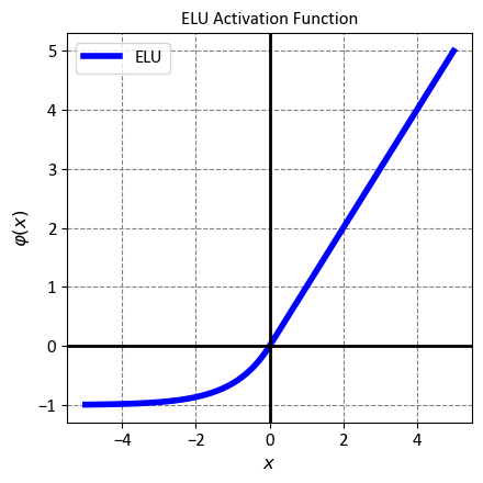
12.2.2.8. Exponential Linear Unit (ELU)#
The Exponential Linear Unit, or ELU for short, is a novel activation function that was proposed to improve the performance and robustness of neural networks. It is a modified version of the Rectified Linear Unit (ReLU) function, meaning it retains the advantages of ReLU while addressing some of its drawbacks. Mathematically, ELU is defined as:
where \(x\) is the input to the function, and \(\alpha\) is a positive constant (typically 1) that controls the behavior of the function for negative inputs. The function can be interpreted as follows:
For positive inputs, ELU behaves like the identity function, meaning it preserves the input value without any change.
For negative inputs, ELU outputs a small negative value that depends on the exponential of the input, resulting in a smooth and non-linear function with a slope of \(\alpha\).
ELU has several benefits over ReLU, such as [Clevert et al., 2015]:
It avoids the dying ReLU problem, where some neurons can stop learning due to zero outputs and gradients. By allowing a small negative output for negative inputs, ELU ensures that the neurons remain active and responsive to the input variations.
It is closer to zero-centered, meaning it has a mean closer to zero. This can prevent a shift in the distribution of the inputs to the next layer, which can improve the learning dynamics and convergence of the model. ELU can create more balanced and stable representations by reducing the input bias to a negative value, which can decrease the correlation and redundancy among the features.
It has a faster learning rate, meaning it can achieve better results in less time and with fewer resources. This is because ELU has a larger and more consistent gradient for both positive and negative inputs, which can accelerate the gradient descent process and reduce the overfitting risk.
Show code cell source
import numpy as np
import matplotlib.pyplot as plt

# Define the ELU function
def elu(x, alpha=1.0):
    return np.where(x > 0, x, alpha * (np.exp(x) - 1))

# Generate x values
x = np.linspace(-5, 5, 100)

# Apply the ELU function to x values
y = elu(x)

# Create the plot using subplots
fig, ax = plt.subplots(figsize=(4.5, 4.5))
_ = ax.plot(x, y, label='ELU', color='blue', linewidth=4)
_ = ax.axhline(0, color='black', linewidth=2, linestyle='-')
_ = ax.axvline(0, color='black', linewidth=2, linestyle='-')
_ = ax.set(xlabel=r'$x$', ylabel= r'$\varphi(x)$',
           title='ELU Activation Function')
_ = ax.legend(fontsize = 12)
_ = ax.grid(True)
plt.tight_layout()
12.2.3. Feedforward and Backpropagation Concepts#
Neural networks, like the intricate workings of our own brains, have a central role in modern machine learning and artificial intelligence. Their ability to process information and learn hinges on the coordinated interplay of two key steps: feedforward and backpropagation.
12.2.3.1. Feedforward#
Feedforward, much like how our senses process information, takes the first step in a neural network’s journey. This process involves these important stages [Erkaymaz, 2020, Maynard, 2020, Yu et al., 2002]:
Input Layer: At the beginning, the input data resides in the input layer. Each neuron here represents a specific feature or characteristic of the data.
Hidden Layers: The real magic unfolds as the data travels through hidden layers. Neurons in these layers interpret inputs from the prior layer, assigning them weights and passing them through an activation function. This transformation introduces non-linear changes, allowing the network to decipher intricate data relationships.
Output Layer: The journey concludes in the output layer, where transformed data takes its final shape—prediction. In tasks like classification, each neuron embodies a class, with the one activated most indicating the network’s decision.
This dance between feedforward and backpropagation embodies the essence of neural network learning, propelling machines to understand, learn, and predict much like our own minds do.
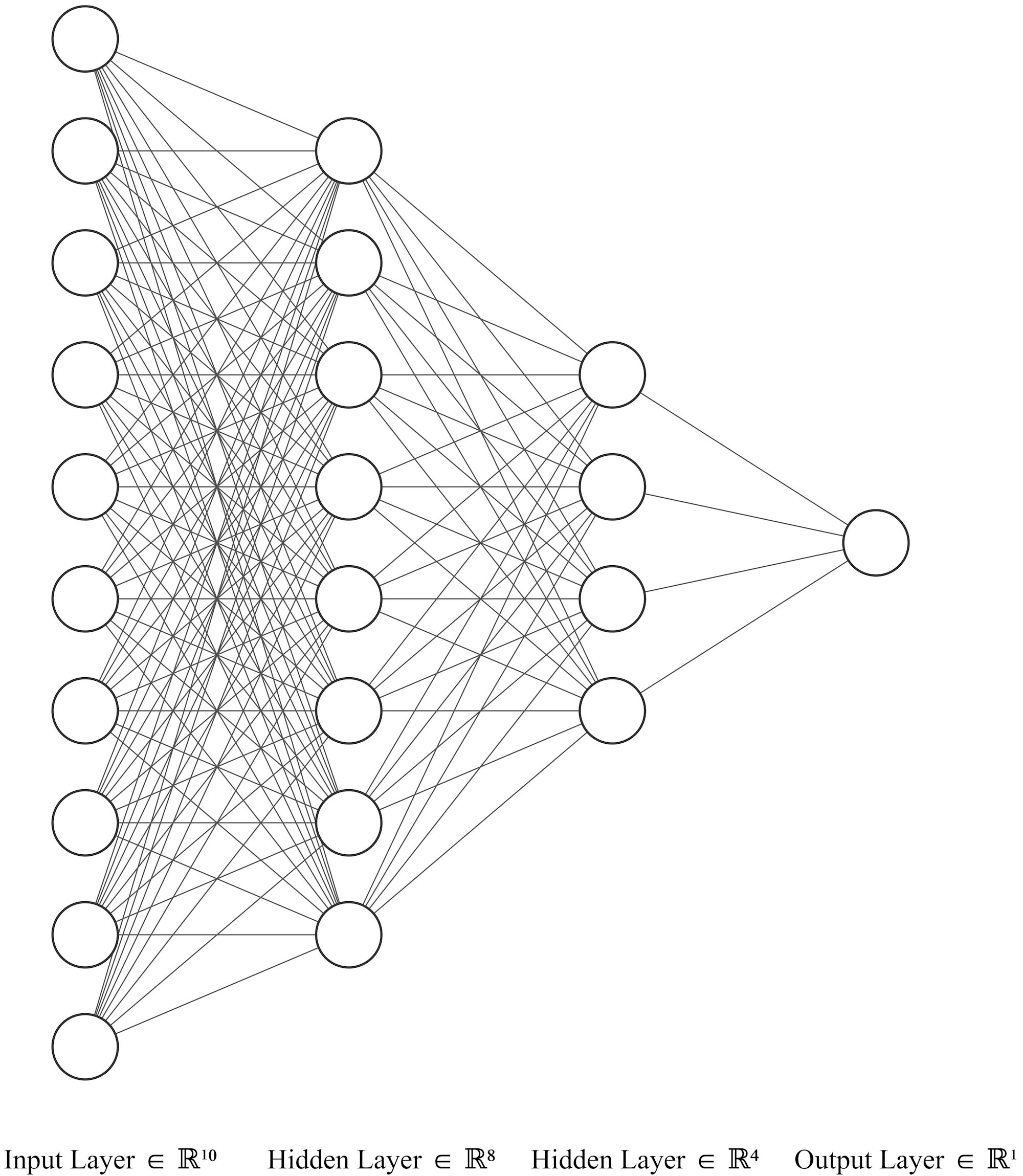
Fig. 12.3 An example of a Neural Metwork: Input, hidden, and output layers.#
12.2.3.2. Backpropagation#
Backpropagation is a powerful algorithm that enables a neural network to learn from its own mistakes and improve its performance over time. It works in tandem with the feedforward process, which passes the input data through the network and generates the output predictions. Backpropagation follows these steps [Erkaymaz, 2020, Maynard, 2020, Yu et al., 2002]:
Loss Calculation: The first step is to measure how well the network is doing by comparing the output predictions with the actual target values. This comparison is done by using a loss function, which quantifies the difference or error between the two. The loss function acts as a feedback signal, indicating how much the network needs to adjust its parameters (weights and biases) to reduce the error.
Gradient Descent: The second step is to find the direction and magnitude of the adjustment for each parameter. This is done by using the gradient, which is the derivative or slope of the loss function with respect to the parameter. The gradient tells us how the loss function changes when we change the parameter slightly. By following the negative gradient, we can find the optimal value of the parameter that minimizes the loss function.
Weight Updates: The third step is to apply the adjustment to each parameter according to the gradient. This is done by using a learning rate, which is a small positive constant that controls the size of the adjustment. The learning rate determines how fast or slow the network learns. By multiplying the gradient by the learning rate, we can obtain the amount of change for each parameter. By subtracting this change from the current value of the parameter, we can update the parameter to a new value that reduces the error.
Iterative Process: The final step is to repeat the above steps for each input-output pair in the data set, and for multiple rounds or epochs. This is an iterative process that gradually improves the network’s accuracy and generalization. With each iteration, the network’s predictions become closer to the target values. The loss function decreases, reflecting the network’s progress and performance.
Through this iterative process of feedforward and backpropagation, the neural network learns to recognize the patterns and relationships hidden in the data. This learning process enables the network to perform various tasks, such as classification, regression, image recognition, natural language processing, and more. As the network learns, it becomes more intelligent and capable, transforming itself from a simple mathematical model to a powerful artificial intelligence system.
12.2.4. Loss Functions in Deep Learning#
Loss functions are essential components of deep learning models, as they provide a way to measure the performance and guide the learning process of the neural networks. They are mathematical functions that compare the output predictions of the network with the actual target values of the data, and quantify the difference or error between them. This error reflects how well or poorly the network is doing its job, and serves as a feedback signal that the network uses to adjust its parameters (weights and biases) and improve its accuracy and generalization [Bishop, 2016, Goodfellow et al., 2016].
12.2.4.1. Why Loss Functions Matter#
Deep learning is the process of creating models that can learn from data and make predictions for new, unseen data. A loss function is a crucial component of this process, as it provides a way to evaluate the quality and accuracy of the model’s predictions. A loss function compares the model’s output predictions with the actual target values of the data, and calculates the difference or error between them. This error reflects how well or poorly the model is performing its task, and serves as a feedback signal that the model uses to improve itself. By using a loss function, the model can adjust its parameters (weights and biases) based on the error, and try to minimize it. Therefore, a loss function acts as a guide that helps the model move in the right direction and achieve better results [Bishop, 2016, Goodfellow et al., 2016, Terven et al., 2023].
12.2.4.2. How Loss Functions Help the Model#
Loss functions are essential components of deep learning models, as they provide a way to measure the performance and guide the learning process of the neural networks. They are mathematical functions that compare the output predictions of the network with the actual target values of the data, and quantify the difference or error between them. This error reflects how well or poorly the network is performing its task, and serves as a feedback signal that the network uses to improve itself. By using a loss function, the network can adjust its parameters (weights and biases) based on the error, and try to minimize it. Therefore, a loss function acts as a guide that helps the network move in the right direction and achieve better results. [Bishop, 2016, Goodfellow et al., 2016]
During training, the network keeps changing its parameters based on the feedback from the loss function. This is done by using an optimization algorithm, such as gradient descent, which calculates the gradient of the loss function with respect to the parameters, and updates the parameters in the opposite direction of the gradient. This process helps the network reduce the error and increase the accuracy of its predictions. As the network trains and updates itself, it gets closer and closer to making predictions that match the target values. [Bishop, 2016, Goodfellow et al., 2016]
In this way, loss functions help models improve over time and learn from their own mistakes. They are crucial for the success and performance of deep learning models, as they define the objective and the direction of the learning process. Different types of loss functions are suitable for different types of tasks and outputs, such as regression, classification, image recognition, natural language processing, and more. [Bishop, 2016, Goodfellow et al., 2016].
12.2.4.3. Popular Loss Functions#
Loss functions are mathematical functions that measure the difference or error between the output predictions of a neural network and the actual target values of the data. They provide a way to evaluate the performance and guide the learning process of the network. Different types of loss functions are suitable for different types of tasks and outputs, such as regression, classification, image recognition, natural language processing, and more. Some of the most common loss functions are [Bishop, 2016, Goodfellow et al., 2016, Terven et al., 2023]:
Mean Squared Error (MSE): This loss function is applied to regression tasks, where the aim is to predict continuous numerical values. It calculates the average of the squared differences between the predicted and actual values. Mathematically, it’s expressed as [Deisenroth et al., 2020, Géron, 2022, Terven et al., 2023]:
where:
\(n\) is the number of data points.
\(y_i\) represents the actual value for the \(i\)th data point.
\(\hat{y}_i\) is the predicted value for the \(i\)th data point.
MSE penalizes large errors more than small errors, and aims to minimize the variance of the predictions.
Binary Cross-Entropy Loss: Used for binary classification tasks, where the aim is to predict the probability of an instance belonging to one of two classes. It quantifies the difference between predicted probabilities and the actual binary labels. Mathematically, it’s given by [Bishop, 2016, Goodfellow et al., 2016, Terven et al., 2023]:
where:
\(n\) is the number of instances.
\(y_i\) is the actual binary label for the \(i\)th instance.
\(p_i\) is the predicted probability of the positive class for the \(i\)th instance.
BCE penalizes incorrect predictions more than correct predictions, and aims to maximize the likelihood of the predictions.
Categorical Cross-Entropy Loss: Suited for multi-class classification problems, where the aim is to predict the probability of an instance belonging to one of several classes. It measures the difference between predicted class probabilities and the true class labels. The formula is [Bishop, 2016, Goodfellow et al., 2016, Terven et al., 2023]:
where:
\(n\) is the number of instances.
\(C\) is the number of classes.
\(y_{ij}\) is an indicator (0 or 1) if instance \(i\) belongs to class \(j\).
\(p_{ij}\) is the predicted probability of instance \(i\) belonging to class \(j\).
CCE penalizes incorrect predictions more than correct predictions, and aims to maximize the likelihood of the predictions.
Sparse Categorical Cross-Entropy Loss: This variation of categorical cross-entropy is useful when true labels are provided as integers, instead of one-hot encoded vectors. It still measures the difference between predicted and actual class probabilities. Mathematically, it’s defined as [Bishop, 2016, Goodfellow et al., 2016, Terven et al., 2023]:
(12.11)#\[\begin{equation} SCCE = -\frac{1}{n} \sum_{i=1}^{n} \log(p_{i, y_i}) \end{equation}\]where:
\( n \) is the number of instances.
\( p_{i, y_i} \) is the predicted probability of instance \( i \) belonging to its true class \( y_i \).
SCCE is computationally more efficient than CCE, as it does not require converting the labels to one-hot vectors.
Hinge Loss (SVM Loss): Primarily used for support vector machines (SVMs) and classification tasks in neural networks. It encourages the correct class scores to be higher than the incorrect class scores by a predefined margin. The hinge loss can be defined as [Cortes and Vapnik, 1995, Rosasco et al., 2004, Terven et al., 2023]:
where \(y_i\) is the actual label (either -1 or 1), and \(\hat{y}_i\) is the predicted score for class \(i\).
Hinge loss penalizes misclassified instances more than correctly classified instances, and aims to maximize the margin between the classes.
Huber Loss: A robust loss function applied in regression tasks. It offers a balance between mean squared error and mean absolute error, which makes it less sensitive to outliers. Mathematically, it’s defined as [Elkan, 2001, Huber, 1992, Terven et al., 2023]:
Where \(\delta\) is a hyperparameter that determines the point where the loss transitions from quadratic to linear behavior.
Huber loss is more robust to outliers than MSE, as it does not square the errors for large values.
Kullback-Leibler Divergence (KL Divergence): Commonly used in generative models like variational autoencoders. It measures the difference between two probability distributions \(P\) and \(Q\) [Cover and Thomas, 2012, Kullback and Leibler, 1951, Terven et al., 2023]:
KL divergence quantifies how much information is lost when using \(Q\) to approximate \(P\). It is also known as the relative entropy.
Triplet Loss: This loss is used in tasks like face recognition and similarity learning. It ensures that embeddings of similar examples are closer in the embedding space than embeddings of dissimilar examples. Mathematically, for a triplet of examples \((a, p, n)\) [Chechik et al., 2010, Schroff et al., 2015, Terven et al., 2023]:
where \(d(x, y)\) measures the distance between embeddings \(x\) and \(y\), and \(\alpha\) is a margin parameter.
Triplet loss minimizes the distance between an anchor example and a positive example, while maximizing the distance between the anchor example and a negative example.
Focal Loss: This loss is used for imbalanced classification problems, where some classes are more frequent than others. It modifies the cross-entropy loss by adding a weighting factor that reduces the loss contribution of easy and well-classified examples, and increases the loss contribution of hard and misclassified examples. Mathematically, for a binary classification problem, it is defined as:
where \(p\) is the predicted probability of the positive class, \(\alpha\) is a balancing factor, and \(\gamma\) is a focusing parameter.
Focal loss reduces the dominance of the majority class and boosts the learning of the minority class. [Lin et al., 2017]
Dice Loss: This loss is used for semantic segmentation tasks, where the aim is to assign a class label to each pixel in an image. It measures the similarity between the predicted and actual segmentation masks, using the Dice coefficient. Mathematically, it is defined as:
where \(y_i\) is the actual binary label for pixel \(i\), \(\hat{y}_i\) is the predicted probability for pixel \(i\), \(n\) is the number of pixels, and \(\epsilon\) is a small constant to avoid division by zero.
Dice loss is robust to class imbalance and can capture the spatial overlap between the masks. [Milletari et al., 2016]
Contrastive Loss: This loss is used for metric learning tasks, where the aim is to learn a distance metric that can measure the similarity or dissimilarity between pairs of examples. It encourages the distance between similar examples to be smaller than the distance between dissimilar examples by a predefined margin. Mathematically, for a pair of examples \((x_1, x_2)\) with a binary label \(y\) indicating their similarity (0 for dissimilar, 1 for similar), it is defined as:
where \(d\) is the Euclidean distance between the embeddings of \(x_1\) and \(x_2\), and \(m\) is the margin parameter.
Contrastive loss can learn meaningful and discriminative embeddings that can be used for tasks like face verification, image retrieval, and clustering. [Hadsell et al., 2006]
12.2.5. Training and Optimization in Deep Learning#
Training and optimizing a neural network is a complex and iterative process that involves adjusting the network’s parameters to learn from data and improve its performance on a specific task. This process is essential for building effective neural networks that can make accurate and meaningful predictions, classifications, and outputs. In this section, we will explore the key steps involved in training and optimizing neural networks. [Bishop, 2016, Goodfellow et al., 2016]
12.2.5.1. The Training Process: Unraveling the Steps#
The journey of training a neural network consists of several fundamental stages, each contributing to the network’s ability to comprehend complex patterns within the data it encounters. These stages can be summarized as follows:
Data Collection & Preprocessing: The process begins with the collection of relevant and appropriately labeled data. High-quality training data is crucial for ensuring the network generalizes well to unseen examples. Data preprocessing, which involves tasks like normalization, scaling, and handling missing values, prepares the data for effective learning. [Bishop, 2016, Goodfellow et al., 2016]
Model Architecture Design: Designing an appropriate model architecture is critical. This step involves defining the structure of the neural network, including the number and arrangement of layers, the type of activation functions used, and how information flows through the network. [Bishop, 2016, Goodfellow et al., 2016]
Initialize Model Parameters: Before training begins, the model’s parameters (weights and biases) are initialized. Proper initialization can set the stage for faster and more stable convergence during optimization. [Glorot and Bengio, 2010, He et al., 2015]
Forward Pass: During the forward pass, input data is fed into the network, and the model generates predictions. This pass involves applying the defined transformations and activation functions layer by layer. [Bishop, 2016, Goodfellow et al., 2016]
Calculate Loss: The generated predictions are compared with the ground truth labels using a predefined loss function. This function quantifies the discrepancy between predictions and actual values. [Bishop, 2016, Goodfellow et al., 2016, Terven et al., 2023]
Backpropagation: Backpropagation involves calculating the gradients of the loss with respect to the model’s parameters. This step enables the network to understand how changes in each parameter affect the overall loss. [LeCun et al., 2015, Rumelhart et al., 1986]
Update Model Parameters: Using the calculated gradients, optimization algorithms like gradient descent are employed to update the model’s parameters. These updates aim to minimize the loss and steer the network towards better performance. [LeCun et al., 2015, Ruder, 2016]
Check Convergence: The training process is performed iteratively. After each iteration (epoch), the convergence of the model is evaluated by monitoring the changes in the loss and other performance metrics. If the model shows signs of convergence or meets predefined criteria, training can stop. [Bishop, 2016, Goodfellow et al., 2016]
Through this iterative process of forward pass, loss calculation, backpropagation, and parameter update, the neural network learns to recognize the patterns and relationships hidden in the data. This learning process enables the network to perform various tasks, such as regression, classification, image recognition, natural language processing, and more. [Bishop, 2016, Goodfellow et al., 2016].
12.2.5.2. Illustrating the Process: A Flowchart Perspective#
To better visualize the intricacies of training and optimization, consider the following flowchart that outlines the sequential steps involved:
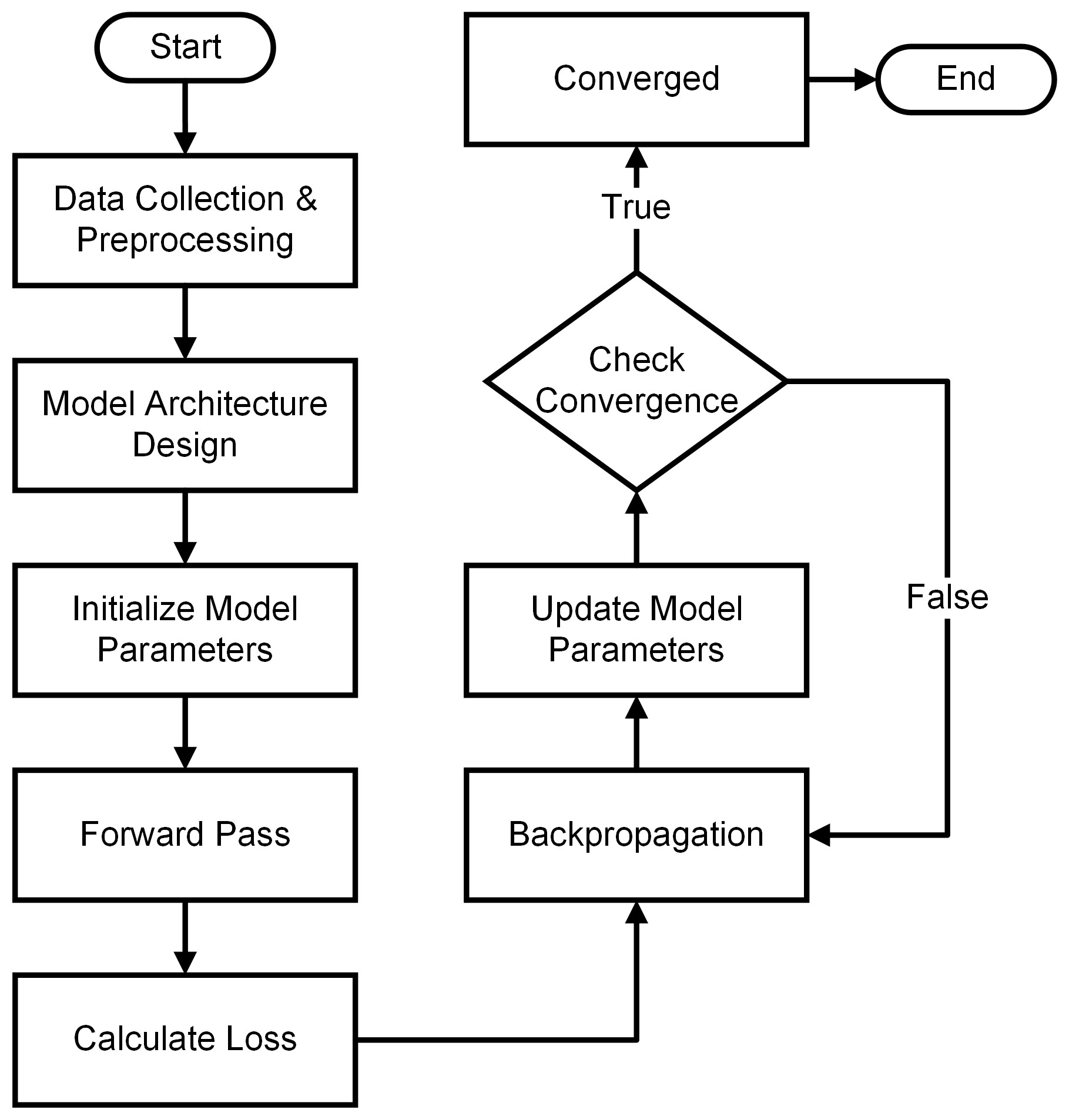
Fig. 12.4 The Structure of Training and Optimization in Deep Learning.#
In this flowchart:
Data Collection & Preprocessing: Gathering and preparing the training data.
Model Architecture Design: Defining the structure of the neural network.
Initialize Model Parameters: Setting initial weights and biases.
Forward Pass: Propagating input data through the network to generate predictions.
Calculate Loss: Comparing predictions to actual values and computing a loss/error metric.
Backpropagation: Calculating gradients of the loss with respect to model parameters.
Update Model Parameters: Adjusting weights and biases using optimization algorithms (e.g., gradient descent).
Check Convergence: Evaluating whether the training process has converged or met a stopping criterion.
Repeat Backpropagation & Update: If convergence is not reached, repeat the backpropagation and parameter update steps.
Converged: Once convergence is achieved, the model is considered trained.
Trained Model: The neural network with optimized parameters.
End: End of the training process.
Note
Please note that deep learning training involves many details and variations, so this flowchart is a simplified representation. Depending on the context and level of detail you want to provide, you can expand each step and include more specific information.
I can help you refine your paragraph. Here is a possible improved version:
12.2.6. Conclusion#
We have reached the end of our exploration of linear models within the realm of deep learning. Linear models offer us a starting point, shedding light on how neural networks make predictions based on data. Yet, as we peer further, it’s clear that life’s complexities demand more than just linear thinking.
To go beyond linear models, we need to understand three crucial components of deep learning: activation functions, loss functions, and optimization techniques. Activation functions add twists and turns to our neural pathways, enabling networks to decipher the intricate patterns hidden in data. Loss functions act as guiding lights, revealing how much our predictions deviate from the truth. Optimization techniques act like sculptors, refining the network’s inner workings and molding it into a more proficient predictor. [Bishop, 2016, Goodfellow et al., 2016]
However, our journey is not confined to linear routes. Deep learning ushers us into the realm of more intricate architectures. These architectures, filled with layers of computations, transform and amplify the information they receive. This expansion leads us to exciting domains – from understanding visual data with convolutional networks [LeCun et al., 2015] to conversing with computers through recurrent networks [Cho et al., 2014] . Moreover, we delve into creative territories, crafting new content with generative models [Goodfellow et al., 2014] and mastering the art of making informed decisions with reinforcement learning [Sutton and Barto, 2018] .
As we conclude this phase of our exploration, it’s important to recognize that our current understanding is but a stepping stone. The landscape of deep learning continues to expand, offering us a plethora of challenges and opportunities. By grasping the essentials, we equip ourselves to navigate this ever-evolving field with confidence and curiosity.