6.3. Pandas Data Selection#
6.3.1. Attribute Access#
You can use attribute-style access to select columns if the column names are valid Python identifiers.
# Access columns as attributes
column_data = df.column_name
Advantages:
Offers convenient and concise syntax for accessing columns as attributes.
Suitable when column names are valid Python identifiers.
Disadvantages:
Limited to accessing columns only; doesn’t support more complex operations.
Example:
import pandas as pd

# Create a DataFrame
data = {'Name': ['Alice', 'Bob', 'Charlie'],
        'Age': [25, 30, 35]}
df = pd.DataFrame(data)

# Original DataFrame
print("Original DataFrame:")
display(df)

# Access the 'Name' column as an attribute
name_column = df.Name

# 'Name' Column
print("\n'Name' Column:")
display(name_column)
Original DataFrame:
| Name | Age | |
|---|---|---|
| 0 | Alice | 25 |
| 1 | Bob | 30 |
| 2 | Charlie | 35 |
'Name' Column:
0      Alice
1        Bob
2    Charlie
Name: Name, dtype: object
Remark
To retrieve the names of all columns within a DataFrame, the method df.columns can be employed. For example, consider the following code snippet:
import pandas as pd

data = {'Name': ['Alice', 'Bob', 'Charlie'],
        'Age': [25, 30, 35]}
df = pd.DataFrame(data)

column_names = df.columns
print(column_names)
Output:
Index(['Name', 'Age'], dtype='object')
6.3.2. loc - Label-Based Indexing:#
The loc method in Pandas allows you to access DataFrame data using labels or boolean array-based indexing. It’s particularly useful for selecting rows and columns based on customized labels or names. This method provides flexibility and intuition in retrieving specific data [Molin and Jee, 2021, Pandas Developers, 2023].
The syntax for using loc is:
df.loc[row_indexer, column_indexer]
row_indexer: Specifies the row labels to select, which can be a single label, a list of labels, a slice, or a boolean array.column_indexer: Specifies the column labels to select, with similar indexing options.
Example:
import pandas as pd

# Create a dictionary for the DataFrame
data = {'Name': ['Alice', 'Bob', 'Charlie'], 'Age': [25, 30, 35]}

# Create a DataFrame with custom index
df = pd.DataFrame(data, index=['ID1', 'ID2', 'ID3'])

# Original DataFrame
print("Original DataFrame:")
display(df)

# Access rows with labels 'ID1' and 'ID3' and all columns
print("\nAccess rows with labels ID1 and ID3 and all columns:")
selected_rows = df.loc[['ID1', 'ID3'], :]
display(selected_rows)

# Access rows based on a condition and specific columns
print("\nAccess rows based on a condition and specific columns:")
conditioned_rows = df.loc[df['Age'] > 30, ['Name', 'Age']]
display(conditioned_rows)
Original DataFrame:
| Name | Age | |
|---|---|---|
| ID1 | Alice | 25 |
| ID2 | Bob | 30 |
| ID3 | Charlie | 35 |
Access rows with labels ID1 and ID3 and all columns:
| Name | Age | |
|---|---|---|
| ID1 | Alice | 25 |
| ID3 | Charlie | 35 |
Access rows based on a condition and specific columns:
| Name | Age | |
|---|---|---|
| ID3 | Charlie | 35 |
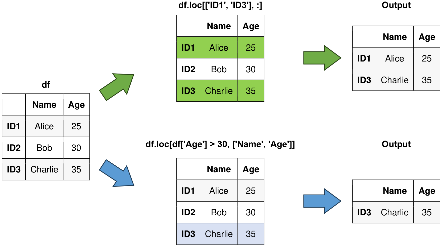
Fig. 6.2 Visual representation of the above example.#
6.3.3. iloc - Position-Based Indexing:#
The iloc method is used for accessing DataFrame data based on integer positions, similar to indexing elements in a Python list. It’s valuable when you want to access data using the underlying integer-based index [Molin and Jee, 2021, Pandas Developers, 2023].
The syntax for using iloc is:
df.iloc[row_indexer, column_indexer]
row_indexer: Specifies the integer positions of the rows to select.column_indexer: Specifies the integer positions of the columns to select.
Example:
import pandas as pd

# Create a dictionary for the DataFrame
data = {'Name': ['Alice', 'Bob', 'Charlie'],
        'Age': [25, 30, 35]}

# Create a DataFrame
df = pd.DataFrame(data)

# Original DataFrame
print("Original DataFrame:")
display(df)

# Access the first two rows and all columns using iloc
print("\nAccess the first two rows and all columns:")
first_two_rows = df.iloc[:2, :]
display(first_two_rows)

# Access specific rows and columns by position using iloc
print("\nAccess specific rows and columns by position:")
selected_rows_columns = df.iloc[[0, 2], [0, 1]]
display(selected_rows_columns)
Original DataFrame:
| Name | Age | |
|---|---|---|
| 0 | Alice | 25 |
| 1 | Bob | 30 |
| 2 | Charlie | 35 |
Access the first two rows and all columns:
| Name | Age | |
|---|---|---|
| 0 | Alice | 25 |
| 1 | Bob | 30 |
Access specific rows and columns by position:
| Name | Age | |
|---|---|---|
| 0 | Alice | 25 |
| 2 | Charlie | 35 |
6.3.4. at - Single Value Selection:#
The at method is ideal for efficiently accessing or modifying a single scalar value in a DataFrame. It offers a direct alternative to loc or iloc for single element selection [Molin and Jee, 2021, Pandas Developers, 2023].
The syntax for using at is:
df.at[row_label, column_label]
row_label: Specifies the label of the row where the desired element is located.column_label: Specifies the label of the column where the element is located.
Advantages:
Allows selection of data from hierarchical structures efficiently.
Provides a clear way to access data at different levels of the index hierarchy.
Disadvantages:
May require an understanding of MultiIndex concepts, which can be complex for newcomers.
Example:
import pandas as pd

# Create a dictionary for the DataFrame
data = {'Name': ['Alice', 'Bob', 'Charlie'],
        'Age': [25, 30, 35]}

# Create a DataFrame
df = pd.DataFrame(data)

# Original DataFrame
print("Original DataFrame:")
display(df)

# Access and modify the element at row label 1 and column label 'Name'
df.at[1, 'Name'] = 'Robert'

# Updated DataFrame
print("\nUpdated DataFrame:")
display(df)

# Access and print the element at row label 2 and column label 'Age'
age = df.at[2, 'Age']
print("\nAge:", age)
Original DataFrame:
| Name | Age | |
|---|---|---|
| 0 | Alice | 25 |
| 1 | Bob | 30 |
| 2 | Charlie | 35 |
Updated DataFrame:
| Name | Age | |
|---|---|---|
| 0 | Alice | 25 |
| 1 | Robert | 30 |
| 2 | Charlie | 35 |
Age: 35
The at method is particularly efficient for single value retrieval or modification.
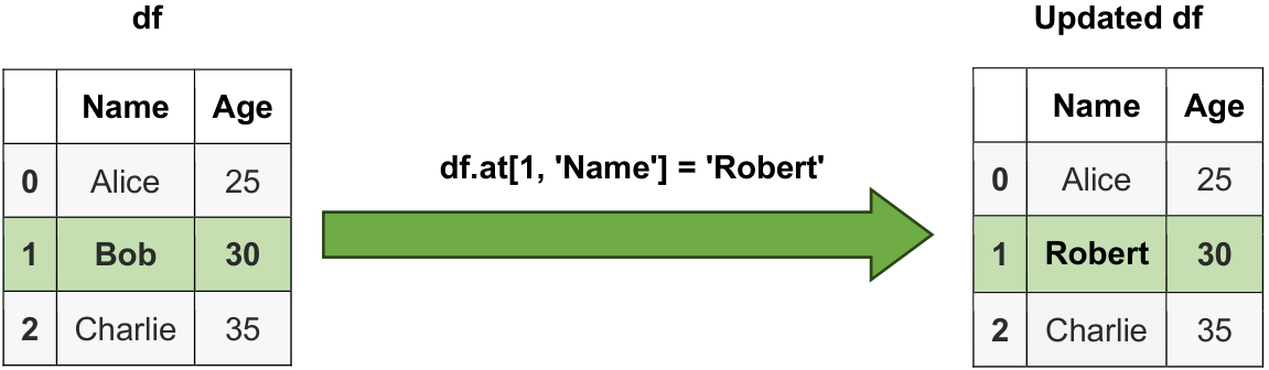
Fig. 6.3 Visual representation of a string.#
6.3.5. Boolean Indexing#
Boolean indexing allows you to select rows based on conditions.
# Select rows where a condition is met
selected_rows = df[df['column'] > value]
You can also use the & (AND) and | (OR) operators for combining conditions.
Advantages:
Simple and intuitive way to filter data based on conditions.
Useful for selecting rows that satisfy specific criteria.
Disadvantages:
Can lead to large intermediate results if conditions are complex.
Not suitable for selecting values based on specific positions.
import pandas as pd

# Create a DataFrame
data = {'Value': [10, 20, 30, 40]}
df = pd.DataFrame(data)

# Original DataFrame
print("Original DataFrame:")
display(df)

# Select rows where the 'Value' column is greater than 20
selected_rows = df[df['Value'] > 20]

# Selected Rows
print("\nSelected Rows:")
display(selected_rows)
Original DataFrame:
| Value | |
|---|---|
| 0 | 10 |
| 1 | 20 |
| 2 | 30 |
| 3 | 40 |
Selected Rows:
| Value | |
|---|---|
| 2 | 30 |
| 3 | 40 |
6.3.6. between() Method#
The pandas.Series.between method is used to determine whether each element in a pandas Series falls within a specified range defined by left and right values. It returns a Boolean Series where each element is True if it falls within the range (inclusive by default) and False if it does not.
pandas.Series.between(left, right, inclusive = 'both')
left: This parameter specifies the left boundary of the range. Elements in the Series are considered within the range if they are greater than or equal to this value.right: This parameter specifies the right boundary of the range. Elements in the Series are considered within the range if they are less than or equal to this value.inclusive: Theinclusiveparameter allows you to specify how the boundaries of the range are treated, and it can take one of the following values:"both": Both the left and right boundaries are included in the range. This means that values equal to theleftandrightparameters are considered within the range."neither": Neither the left nor the right boundaries are included in the range. Values equal to theleftandrightparameters are not considered within the range."left": Only the left boundary is included in the range. Values equal to theleftparameter are considered within the range, but values equal to therightparameter are not."right": Only the right boundary is included in the range. Values equal to therightparameter are considered within the range, but values equal to theleftparameter are not.
This flexibility in specifying how boundaries are treated makes the inclusive parameter a powerful tool when using the pandas.Series.between function for data filtering and categorization.
You can see the full syntax here.
Advantages:
Provides a convenient way to filter and categorize data within a specified range.
Supports both inclusive and exclusive range definitions, allowing flexibility in data selection.
Returns a Boolean Series, which can be easily used for conditional filtering and further analysis.
Disadvantages:
It may not be as efficient for large datasets compared to other filtering methods that use vectorized operations.
Example:
import pandas as pd

# Create a pandas DataFrame representing temperature measurements in degrees Celsius
temperature_data = pd.DataFrame({'Temperature': [20, 25, 30, 35, 40, 45, 50, 55]})

# Print the original temperature data DataFrame
print("Original Temperature Data:")
display(temperature_data)

# Check if temperatures fall within the range [25, 45] (inclusive)
inclusive_both = temperature_data['Temperature'].between(25, 45, inclusive="both")

# Print the Boolean Series indicating whether temperatures are within the range [25, 45]
print("\nBoolean Series for Inclusive Range [25, 45] (inclusive):")
print(inclusive_both)

# Use the Boolean Series to filter and display temperatures within the specified range
filtered_temperatures = temperature_data.loc[inclusive_both]

# Print the filtered temperatures DataFrame
print("\nFiltered Temperatures within the Inclusive Range [25, 45]:")
display(filtered_temperatures)
Original Temperature Data:
| Temperature | |
|---|---|
| 0 | 20 |
| 1 | 25 |
| 2 | 30 |
| 3 | 35 |
| 4 | 40 |
| 5 | 45 |
| 6 | 50 |
| 7 | 55 |
Boolean Series for Inclusive Range [25, 45] (inclusive):
0    False
1     True
2     True
3     True
4     True
5     True
6    False
7    False
Name: Temperature, dtype: bool

Filtered Temperatures within the Inclusive Range [25, 45]:
| Temperature | |
|---|---|
| 1 | 25 |
| 2 | 30 |
| 3 | 35 |
| 4 | 40 |
| 5 | 45 |
6.3.7. query() Method#
The query() method allows you to write complex queries using a more concise syntax.
# Using query() to filter data
result = df.query(expr)
You can see the full syntax here.
Advantages:
Allows writing complex queries using a more readable and concise syntax.
Reduces the need for nested parentheses when filtering with multiple conditions.
Disadvantages:
May require an understanding of query language and its limitations.
Slightly slower than direct indexing or boolean indexing for simple conditions.
Example:
import pandas as pd

# Create a DataFrame
data = {'Value1': [10, 20, 30, 40],
        'Value2': [5, 15, 25, 35]}
df = pd.DataFrame(data)

# Original DataFrame
print("Original DataFrame:")
display(df)

# Use the query() method to filter data
result = df.query("Value1 > 20 and Value2 == 35")

# Filtered Result
print("\nFiltered Result:")
display(result)
Original DataFrame:
| Value1 | Value2 | |
|---|---|---|
| 0 | 10 | 5 |
| 1 | 20 | 15 |
| 2 | 30 | 25 |
| 3 | 40 | 35 |
Filtered Result:
| Value1 | Value2 | |
|---|---|---|
| 3 | 40 | 35 |
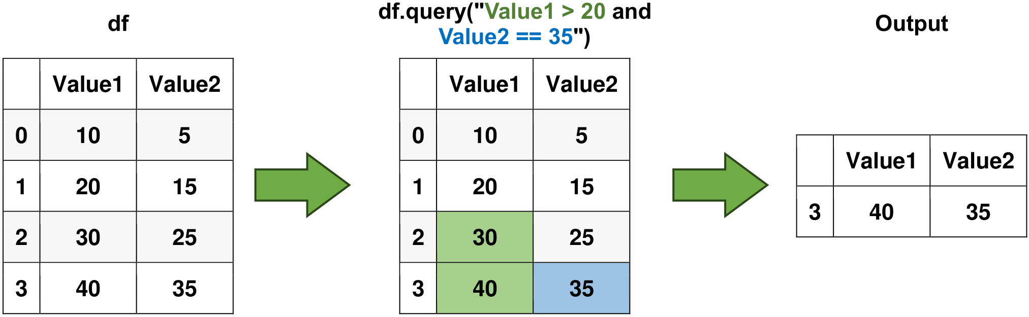
Fig. 6.4 Visual representation of the above example.#
6.3.8. isin() Method#
The isin() method allows you to filter data based on values in a list.
# Filtering using isin() method
selected_rows = df[df['column'].isin([value1, value2])]
Advantages:
Efficient way to filter data based on multiple values in a column.
Useful for scenarios where you need to extract rows with specific values.
Disadvantages:
Limited to filtering based on a predefined list of values.
Not suitable for complex conditions involving multiple columns.
Example:
import pandas as pd

# Create a DataFrame
data = {'Category': ['A', 'B', 'C', 'A', 'B', 'C']}
df = pd.DataFrame(data)

# Original DataFrame
print("Original DataFrame:")
display(df)

# Use isin() to filter data
selected_rows = df[df['Category'].isin(['A', 'C'])]

# Selected Rows
print("\nSelected Rows:")
display(selected_rows)
Original DataFrame:
| Category | |
|---|---|
| 0 | A |
| 1 | B |
| 2 | C |
| 3 | A |
| 4 | B |
| 5 | C |
Selected Rows:
| Category | |
|---|---|
| 0 | A |
| 2 | C |
| 3 | A |
| 5 | C |
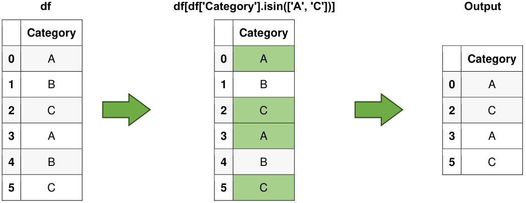
Fig. 6.5 Visual representation of the above example.#
6.3.9. xs() Method#
The xs() method allows you to cross-section data from a DataFrame, particularly useful for MultiIndex DataFrames.
# Cross-section data from a MultiIndex DataFrame
result = df.xs(key, level='index_level')
Advantages:
Facilitates cross-sectional data extraction from MultiIndex DataFrames.
Useful for scenarios where you need to access data from specific levels of the index hierarchy.
Disadvantages:
Limited to cross-sections; might not cover all MultiIndex data selection needs.
Requires familiarity with MultiIndex structure.
Example:
import pandas as pd

# Create a MultiIndex DataFrame
data = {'Value': [10, 20, 30, 40]}
index = pd.MultiIndex.from_tuples([('A', 'X'), ('A', 'Y'), ('B', 'X'), ('B', 'Y')],
                                  names=['Index1', 'Index2'])
df = pd.DataFrame(data, index=index)

# Original MultiIndex DataFrame
print("Original MultiIndex DataFrame:")
display(df)

# Use xs() to cross-section data
result = df.xs('X', level='Index2')

# Selected Rows
print("\nSelected Rows:")
display(result)
Original MultiIndex DataFrame:
| Value | ||
|---|---|---|
| Index1 | Index2 | |
| A | X | 10 |
| Y | 20 | |
| B | X | 30 |
| Y | 40 |
Selected Rows:
| Value | |
|---|---|
| Index1 | |
| A | 10 |
| B | 30 |
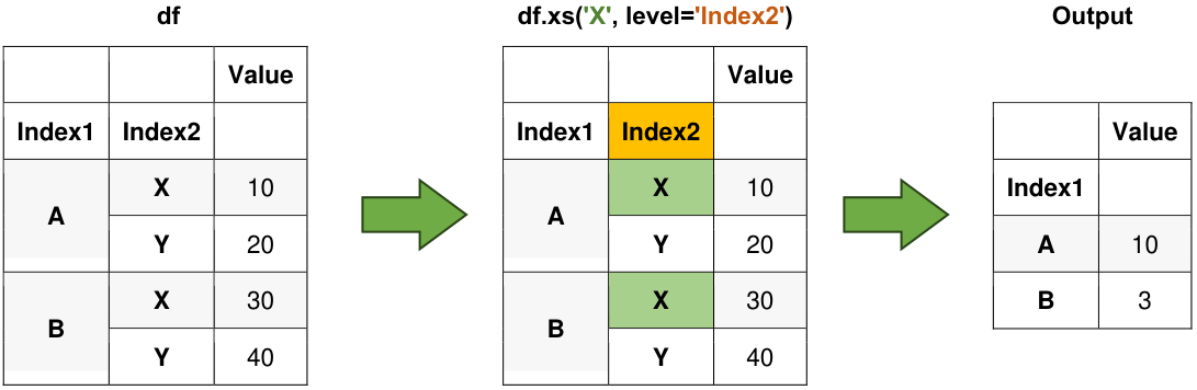
Fig. 6.6 Visual representation of the above example.#
6.3.10. get() Method#
The get() method allows you to access values using default values for missing keys or labels.
# Using get() to access data with default value
value = df.get(label, default_value)
Advantages:
Provides a way to access values with a default value if the label is missing.
Useful for handling missing keys or labels without raising exceptions.
Disadvantages:
Limited to single-value access; not suitable for more complex selection needs.
Might lead to inconsistent behavior if used excessively.
import pandas as pd

# Create a DataFrame
data = {'Name': ['Alice', 'Bob', 'Charlie'],
        'Age': [25, 30, 35]}
df = pd.DataFrame(data)

# Original DataFrame
print("Original DataFrame:")
display(df)

# Use get() to access data with a default value
value = df.get('City', default='Unknown')

# Retrieved Values
print("\nRetrieved Values:")
print(value)
Original DataFrame:
| Name | Age | |
|---|---|---|
| 0 | Alice | 25 |
| 1 | Bob | 30 |
| 2 | Charlie | 35 |
Retrieved Values:
Unknown
6.3.11. where() Method#
The where() method returns a DataFrame with the same shape as the original but with NaNs where the condition is not met.
# Using where() to filter data conditionally
filtered_df = df.where(df['column'] > value)
You can see the full syntax here.
Advantages:
Retains the original shape of the DataFrame, replacing values where the condition is not met.
Useful for creating a masked array with NaN values where the condition is False.
Disadvantages:
Creates a new DataFrame with NaN values, potentially leading to memory overhead.
Might not be suitable for cases where you want to remove rows based on conditions.
import pandas as pd

# Create a DataFrame
data = {'Value': [10, 20, 30, 40]}
df = pd.DataFrame(data)

# Original DataFrame
print("Original DataFrame:")
display(df)

# Use where() to filter data conditionally
filtered_df = df.where(df['Value'] > 20, other=pd.NA)

# Filtered Data
print("\nFiltered Data:")
display(filtered_df)
Original DataFrame:
| Value | |
|---|---|
| 0 | 10 |
| 1 | 20 |
| 2 | 30 |
| 3 | 40 |
Filtered Data:
| Value | |
|---|---|
| 0 | NaN |
| 1 | NaN |
| 2 | 30.0 |
| 3 | 40.0 |
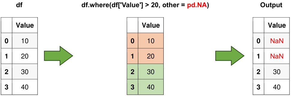
Fig. 6.7 Visual representation of the above example.#
Note
It is worth noting that the concept of
pd.NAin the context of the Pandas library is akin tonp.nanfrom the NumPy library. Bothpd.NAandnp.nanare used to represent missing or undefined values within data structures. These sentinel values serve the purpose of indicating the absence of a valid numeric or data entry at a particular location in a dataset.The
DataFrame.where()function exhibits a distinct signature when compared tonumpy.where(). Specifically, the expression df1.where(m, df2) can be regarded as analogous tonumpy.where(m, df1, df2)[Pandas Developers, 2023].
Example - pandas.DataFrame.where for series:
import pandas as pd

# Create a pandas DataFrame representing temperature measurements in degrees Celsius
temperature_data = pd.Series([-10, -15, -12.5, -13, -2, -5, -1, 10, 15, 12, 13.5, 14, 14.5, 5, 5])

# Use the DataFrame.where() function to filter temperatures greater than 0
temperature_data.where(temperature_data > 0)
0      NaN
1      NaN
2      NaN
3      NaN
4      NaN
5      NaN
6      NaN
7     10.0
8     15.0
9     12.0
10    13.5
11    14.0
12    14.5
13     5.0
14     5.0
dtype: float64
The pandas.DataFrame.mask function is employed to substitute values when a specified condition is met. For further information, please refer to this link.
import pandas as pd

# Create a pandas DataFrame representing temperature measurements in degrees Celsius
temperature_data = pd.Series([-10, -15, -12.5, -13, -2, -5, -1, 10, 15, 12, 13.5, 14, 14.5, 5, 5])

# Apply the DataFrame.mask() function to replace values where the condition is True (temperatures greater than 0)
temperature_data.mask(temperature_data > 0)
0    -10.0
1    -15.0
2    -12.5
3    -13.0
4     -2.0
5     -5.0
6     -1.0
7      NaN
8      NaN
9      NaN
10     NaN
11     NaN
12     NaN
13     NaN
14     NaN
dtype: float64
6.3.12. query() Method with Variables (Optional Content)#
You can use variables in the query() method by prefixing them with the @ symbol.
# Using variables in query() method
age_threshold = 30
result = df.query("Age > @age_threshold")
Advantages:
Enables parameterized queries using external variables for improved readability.
Useful for scenarios where you need to reuse the same condition with different values.
Disadvantages:
Variables must be prefixed with the
@symbol, which can be confusing for newcomers.Might not be the most efficient option for extremely complex conditions.
import pandas as pd

# Create a DataFrame
data = {'Age': [25, 30, 35, 40]}
df = pd.DataFrame(data)

# Original DataFrame
print("Original DataFrame:")
display(df)

# Use variables in query() method
age_threshold = 30
result = df.query("Age > @age_threshold")

# Filtered Result
print("\nFiltered Result:")
display(result)
Original DataFrame:
| Age | |
|---|---|
| 0 | 25 |
| 1 | 30 |
| 2 | 35 |
| 3 | 40 |
Filtered Result:
| Age | |
|---|---|
| 2 | 35 |
| 3 | 40 |