5.1. Basics of Numpy#
5.1.1. Installation#
NumPy is not a built-in library in Python, so you need to install it separately. You can use pip, the Python package manager, to install NumPy:
>>> pip install numpy
Remark
Google Colab (Colaboratory) is a cloud-based Jupyter notebook environment provided by Google, and it comes with a variety of popular data science libraries preinstalled, including NumPy, Pandas, Matplotlib, and more.
5.1.2. Importing NumPy#
To use NumPy in your Python script or interactive session, you need to import it first:
import numpy as np
A common convention is to import NumPy library as “np” for brevity.
5.1.3. Creating NumPy Arrays#
NumPy’s primary data structure is the ndarray (N-dimensional array). You can create a NumPy array using various methods, such as:
import numpy as np
from pprint import pprint  # Importing the pprint module for pretty printing

# Creating arrays from different sources

# From a list or tuple
arr1 = np.array([1, 2, 3, 4, 5])
print("Array from list/tuple:")
pprint(arr1)
Array from list/tuple:
array([1, 2, 3, 4, 5])
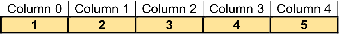
Fig. 5.1 Visualizing np.array([1, 2, 3, 4, 5]).#
# From nested lists
arr2 = np.array([[1, 2, 3], [4, 5, 6]])
print("Array from nested lists:")
pprint(arr2)
Array from nested lists:
array([[1, 2, 3],
       [4, 5, 6]])
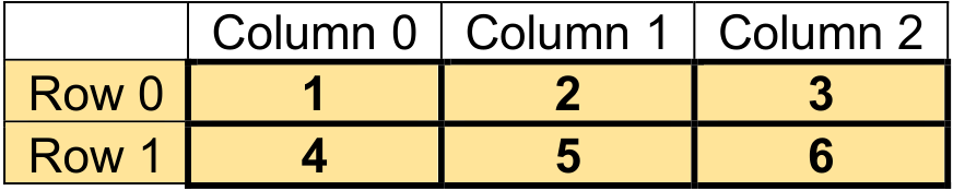
Fig. 5.2 Visualizing np.array([[1, 2, 3], [4, 5, 6]]).#
# Using built-in functions
zeros_arr = np.zeros((3, 4), dtype = 'int16')    # Creates a 3x4 array of zeros
print("Array of zeros:")
pprint(zeros_arr)
Array of zeros:
array([[0, 0, 0, 0],
       [0, 0, 0, 0],
       [0, 0, 0, 0]], dtype=int16)
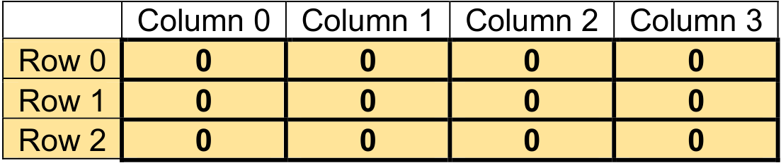
Fig. 5.3 Visualizing np.zeros((3, 4), dtype = ‘int16’).#
ones_arr = np.ones((2, 3), dtype = 'int16')      # Creates a 2x3 array of ones
print("Array of ones:")
pprint(ones_arr)
Array of ones:
array([[1, 1, 1],
       [1, 1, 1]], dtype=int16)
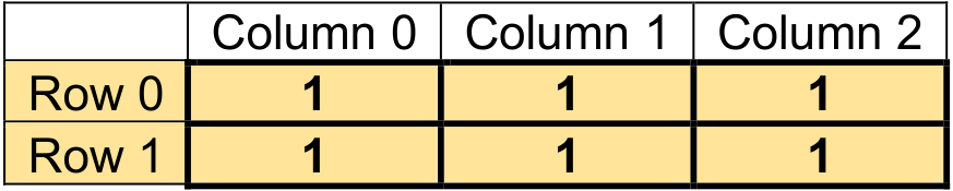
Fig. 5.4 Visualizing np.ones((2, 3), dtype = ‘int16’).#
random_arr = np.random.rand(3, 3)  # Creates a 3x3 array of random values between 0 and 1
print("Array of random values between 0 and 1:")
pprint(random_arr)
Array of random values between 0 and 1:
array([[0.27379993, 0.84370383, 0.67858298],
       [0.8581197 , 0.0343177 , 0.47417405],
       [0.53714247, 0.50349276, 0.16619218]])
5.1.4. Indexing and Slicing#
One of the fundamental strengths of NumPy arrays lies in their versatility when it comes to accessing specific elements or subarrays. Utilizing indexing and slicing, you can navigate through the array’s contents efficiently and precisely. These techniques are essential for extracting data, performing operations on subsets, and manipulating arrays to suit your needs [Harris et al., 2020, NumPy Developers, 2023].
Example:
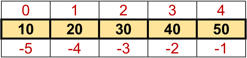
Fig. 5.5 Visualizing np.array([10, 20, 30, 40, 50]).#
def print_bold(txt):
    print("\033[1m" + txt + "\033[0m")

# Creating an array
arr = np.array([10, 20, 30, 40, 50])

# Accessing elements
element_at_index_0 = arr[0]   # Output: 10
element_at_last_index = arr[-1]  # Output: 50

print_bold("Accessing elements:")
pprint(f"Element at index 0: {element_at_index_0}")
pprint(f"Element at last index: {element_at_last_index}")

# Slicing
sliced_arr = arr[1:4] # Output: [20, 30, 40]

print_bold("\nSlicing:")
pprint(sliced_arr)
Accessing elements:
'Element at index 0: 10'
'Element at last index: 50'

Slicing:
array([20, 30, 40])
5.1.5. Shape and Reshaping#
In NumPy, array manipulation is a powerful tool for transforming and optimizing data structures. Understanding the shape of an array and being able to reshape it are essential skills in array manipulation. NumPy offers methods that allow you to seamlessly retrieve the shape of an array and reshape it according to your needs [Harris et al., 2020, NumPy Developers, 2023].
Example:
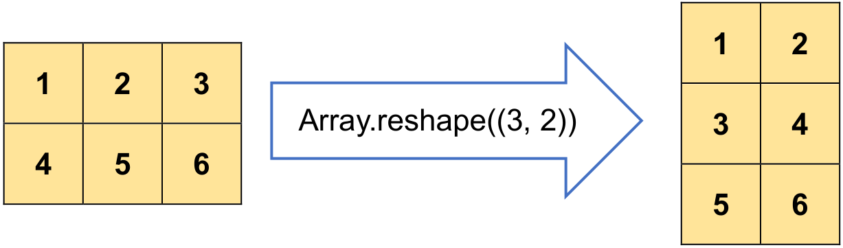
Fig. 5.6 Visualizing Arr.reshape((3, 2)) where Arr = np.array([[1, 2, 3], [4, 5, 6]]).#
# Creating a 2D array
Arr = np.array([[1, 2, 3], [4, 5, 6]])

# Printing the size (shape) of the array
print_bold("Size of the Array:")
pprint(Arr.shape)

# Displaying the original array
print_bold("\nOriginal Array:")
pprint(Arr)

# Reshaping the array
Reshaped_Arr = Arr.reshape((3, 2))

print_bold("\nReshaped Array:")
pprint(Reshaped_Arr)
Size of the Array:
(2, 3)

Original Array:
array([[1, 2, 3],
       [4, 5, 6]])

Reshaped Array:
array([[1, 2],
       [3, 4],
       [5, 6]])
5.1.6. Adding, removing, and sorting elements#
In NumPy, you can easily add, remove, and sort elements in an array using various built-in functions and methods. Here’s a brief explanation of each operation [Harris et al., 2020, NumPy Developers, 2023]:
5.1.6.1. Adding Elements#
To add elements to a NumPy array, you can use functions like numpy.append() or numpy.concatenate().
a. numpy.append(): This function appends elements to the end of an array. It creates a new array with the appended elements.
Example:
# Creating an array
arr = np.array([1, 2, 3])

# Adding a new element
new_element = 4
new_arr = np.append(arr, new_element)

print_bold("Original Array:")
pprint(arr)

print_bold("\nNew Array after Appending:")
pprint(new_arr)  # Output: [1 2 3 4]
Original Array:
array([1, 2, 3])

New Array after Appending:
array([1, 2, 3, 4])
b. numpy.concatenate(): This function concatenates two or more arrays along a specified axis.
Example:
# Creating arrays
arr1 = np.array([1, 2, 3])
arr2 = np.array([4, 5])

# Combining arrays using concatenate
combined_arr = np.concatenate((arr1, arr2))

print_bold("Original Arrays:")
pprint(arr1)
pprint(arr2)

print_bold("\nCombined Array:")
pprint(combined_arr)  # Output: [1 2 3 4 5]
Original Arrays:
array([1, 2, 3])
array([4, 5])

Combined Array:
array([1, 2, 3, 4, 5])
5.1.6.2. Removing Elements#
To remove elements from a NumPy array, you can use functions like numpy.delete() or filter the array based on certain conditions.
a. numpy.delete(): This function removes elements from an array along a specified axis.
Example:
# Creating an array
arr = np.array([1, 2, 3, 4, 5])

# Removing an element by index
index_to_remove = 2
new_arr = np.delete(arr, index_to_remove)

print_bold("Original Array:")
pprint(arr)

print_bold("\nNew Array after Deleting:")
pprint(new_arr)  # Output: [1 2 4 5]
Original Array:
array([1, 2, 3, 4, 5])

New Array after Deleting:
array([1, 2, 4, 5])
b. Filtering with Conditions: You can use boolean indexing to remove elements based on certain conditions.
Example:
# Creating an array
arr = np.array([1, 2, 3, 4, 5])

# Creating a condition to filter elements
condition = arr != 3

# Applying the condition to create a new array
new_arr = arr[condition]

print_bold("Original Array:")
pprint(arr)

print_bold("\nNew Array after Filtering:")
pprint(new_arr)  # Output: [1 2 4 5]
Original Array:
array([1, 2, 3, 4, 5])

New Array after Filtering:
array([1, 2, 4, 5])
5.1.6.3. Sorting Elements#
To sort elements in a NumPy array, you can use the numpy.sort() function.
Example:
# Creating an array
arr = np.array([3, 1, 5, 2, 4])

# Sorting the array
sorted_arr = np.sort(arr)

print_bold("Original Array:")
pprint(arr)

print_bold("\nSorted Array:")
pprint(sorted_arr)  # Output: [1 2 3 4 5]
Original Array:
array([3, 1, 5, 2, 4])

Sorted Array:
array([1, 2, 3, 4, 5])
Keep in mind that the above operations usually create a new array, so if you want to modify the original array in place, you can use appropriate assignment statements.
5.1.7. Multi-dimensional arrays in NumPy#
NumPy employs “ndarrays,” which are multi-dimensional arrays, denoting “N-dimensional arrays.” They serve as the cornerstone data structure for numerical computations within the library and excel in efficiently managing multi-dimensional data. With the capability to possess any number of dimensions, ndarrays facilitate working with diverse data shapes like vectors, matrices, or higher-dimensional arrays.
Diverse functions in NumPy enable the creation of multi-dimensional arrays, including numpy.array(), numpy.zeros(), numpy.ones(), and numpy.random.rand(), among several others [Harris et al., 2020, NumPy Developers, 2023].
5.1.7.1. Creating a 1-dimensional array#
# Creating a 1D array
arr_1d = np.array([1, 2, 3, 4, 5])

print_bold("1D Array:")
pprint(arr_1d)
# Output: [1 2 3 4 5]
1D Array:
array([1, 2, 3, 4, 5])

Fig. 5.7 Visualizing np.array([1, 2, 3, 4, 5]).#
5.1.7.2. Creating a 2-dimensional array (matrix)#
# Creating a 2D array (matrix)
matrix_2d = np.array([[1, 2, 3], [4, 5, 6], [7, 8, 9]])

print_bold("2D Array (Matrix):")
pprint(matrix_2d)
2D Array (Matrix):
array([[1, 2, 3],
       [4, 5, 6],
       [7, 8, 9]])
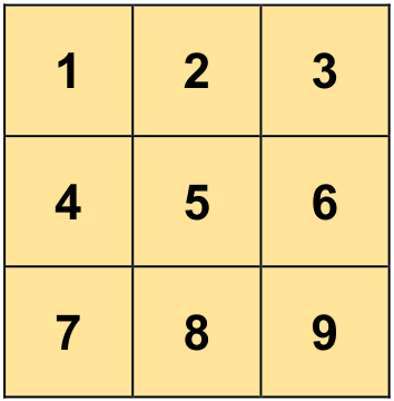
Fig. 5.8 Visualizing np.array([[1, 2, 3], [4, 5, 6], [7, 8, 9]]).#
5.1.7.3. Creating a 3-dimensional array#
# Creating a 3D array (matrix)
matrix_3d = np.array([[[1, 2], [3, 4]],
                      [[5, 6], [7, 8]]])

print_bold("3D Array (Matrix):")
pprint(matrix_3d)
3D Array (Matrix):
array([[[1, 2],
        [3, 4]],

       [[5, 6],
        [7, 8]]])
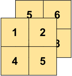
Fig. 5.9 Visualizing np.array([[[1, 2], [3, 4]],[[5, 6], [7, 8]]]).#
You can access elements of multi-dimensional arrays using indexing, similar to regular Python lists. The number of indices you provide corresponds to the number of dimensions of the array.
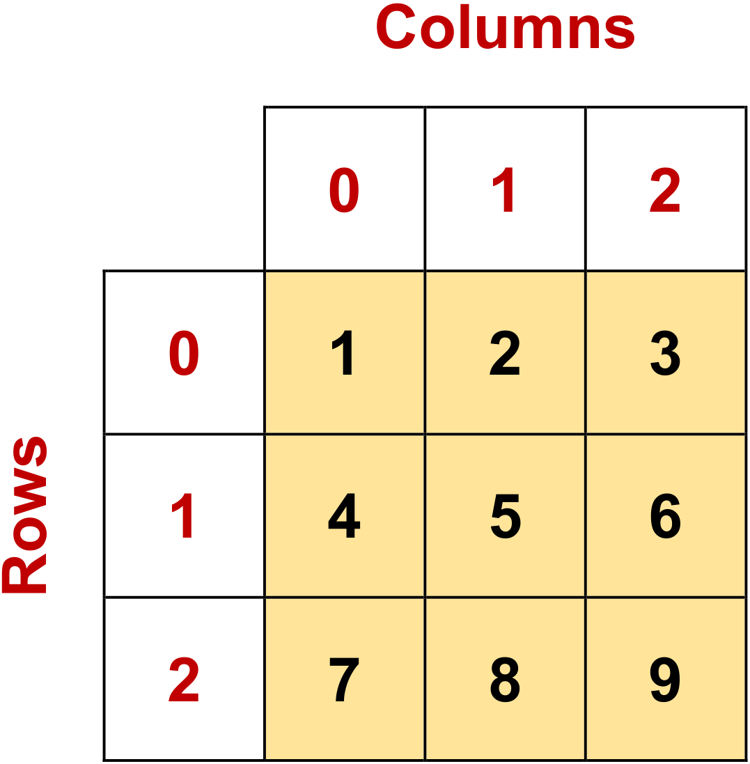
Fig. 5.10 Visualizing np.array([[1, 2, 3], [4, 5, 6], [7, 8, 9]]).#
# Create a 2D NumPy matrix
matrix_2d = np.array([
    [1, 2, 3],
    [4, 5, 6],
    [7, 8, 9]
])

print_bold("2D Matrix:")
pprint(matrix_2d)  # Pretty print the entire matrix

print_bold("\nElement at Row 0, Column 1:")
print(matrix_2d[0, 1])  # Output: 2

print_bold("\nElement at Row 1, Column 1:")
print(matrix_2d[1, 1])  # Output: 5

print_bold("\nRow 0:")
print(matrix_2d[0])  # Output: [1 2 3]

print_bold("\nColumn 1:")
print(matrix_2d[:, 1])  # Output: [2 5 8]
2D Matrix:
array([[1, 2, 3],
       [4, 5, 6],
       [7, 8, 9]])

Element at Row 0, Column 1:
2

Element at Row 1, Column 1:
5

Row 0:
[1 2 3]

Column 1:
[2 5 8]
NumPy also offers numerous functions for manipulating multi-dimensional arrays, including reshaping, slicing, mathematical operations, matrix operations, and more. Its capabilities are essential for scientific computing, data analysis, and machine learning tasks where multi-dimensional data is prevalent.
5.1.8. Convert a 1D array into a 2D array#
You can convert a 1D array into a 2D array in NumPy by adding a new axis using the numpy.newaxis attribute or the numpy.expand_dims() function. Both approaches achieve the same result of increasing the array’s dimensions from 1D to 2D.
5.1.8.1. Using numpy.newaxis#
numpy.newaxis is a special attribute in NumPy that allows you to increase the dimensions of an array by adding a new axis. It is also represented by None. This new axis effectively converts a 1D array into a 2D array, a 2D array into a 3D array, and so on, depending on how many newaxis attributes you add [Harris et al., 2020, NumPy Developers, 2023].
When you use numpy.newaxis in slicing operations, it adds a new axis at the specified position, effectively increasing the number of dimensions by one. This is particularly useful when you want to perform operations that require arrays with different dimensions to be compatible [Harris et al., 2020, NumPy Developers, 2023].
Here’s how numpy.newaxis works with an example:
# Import the necessary library
import numpy as np

# Create a 1D NumPy array
arr_1d = np.array([1, 2, 3, 4, 5])

# Display the 1D array
print_bold("1D Array:")
pprint(arr_1d)

# Calculate and display the shape of the 1D array
print_bold("\nThe shape of 1D Array:")
print(f'Shape: {arr_1d.shape}')

# Convert the 1D array to a 2D array with a new axis
arr_2d = arr_1d[:, np.newaxis]

# Display the resulting 2D array
print_bold("\n2D Array:")
pprint(arr_2d)

# Calculate and display the shape of the 2D array
print_bold("\nThe shape of 2D Array:")
print(f'Shape: {arr_2d.shape}')
1D Array:
array([1, 2, 3, 4, 5])

The shape of 1D Array:
Shape: (5,)

2D Array:
array([[1],
       [2],
       [3],
       [4],
       [5]])

The shape of 2D Array:
Shape: (5, 1)
5.1.8.2. Using numpy.expand_dims()#
numpy.expand_dims() is a function in NumPy that allows you to increase the dimensions of an array by inserting a new axis at a specified position. It is used to reshape arrays and increase their dimensionality. The function is quite flexible and can be used to add a new axis at any desired position.
Here’s the syntax for numpy.expand_dims():
numpy.expand_dims(a, axis)
Parameters:
a: The input array to which a new axis will be added.axis: The position along which the new axis will be inserted. The axis parameter should be an integer or a tuple of integers. Here’s an example of usingnumpy.expand_dims():
# Import the necessary library
import numpy as np

# Create a 1D NumPy array
arr_1d = np.array([1, 2, 3, 4, 5])

# Display the 1D array
print_bold("1D Array:")
pprint(arr_1d)

# Calculate and display the shape of the 1D array
print_bold("\nThe shape of 1D Array:")
print(f'Shape: {arr_1d.shape}')

# Convert the 1D array to a 2D array using np.expand_dims
arr_2d = np.expand_dims(arr_1d, axis=1)

# Display the resulting 2D array
print_bold("\n2D Array:")
print(arr_2d)

# Print the shape of arr_2d
print("\nShape of arr_2d:", arr_2d.shape)

# Access and print elements of the 2D array
print("Element at [row 2, column 0] = ", arr_2d[2, 0])
1D Array:
array([1, 2, 3, 4, 5])

The shape of 1D Array:
Shape: (5,)

2D Array:
[[1]
 [2]
 [3]
 [4]
 [5]]

Shape of arr_2d: (5, 1)
Element at [row 2, column 0] =  3
In this example, arr_1d is a 1D array with shape (5,). Using np.expand_dims(arr_1d, axis=1), we add a new axis at position axis=1, resulting in arr_2d, a 2D array with shape (5, 1). The new axis has been inserted as a new dimension along the vertical direction, converting the 1D array into a column vector.
numpy.expand_dims() is useful when you need to reshape arrays to make them compatible for certain operations or to bring them to a specific shape required by algorithms or functions.
5.1.9. Exploring NumPy’s Versatile Indexing#
NumPy offers a range of advanced indexing and index tricks that provide users with powerful tools to access and manipulate specific elements or subarrays within arrays, utilizing arrays as indices. These features go beyond standard indexing, granting greater flexibility and control. Let’s delve into some examples to better understand their capabilities [NumPy Developers, 2023].
Advanced indexing in NumPy empowers you to utilize arrays or tuples as indices, enabling you to retrieve particular elements or subarrays from the array. Within advanced indexing, there are two main types: integer array indexing and Boolean array indexing. Both methods open up new possibilities for array manipulation and data extraction.
Example - Integer Array Indexing:
Fig. 5.11 Visualizing np.array([10, 20, 30, 40, 50]).#
# Create a NumPy array
data = np.array([10, 20, 30, 40, 50])

# Create an array of indices to select elements
indices = np.array([0, 2, 4])

# Use integer array indexing to select specific elements
selected_elements = data[indices]

print_bold("Selected Elements:")
pprint(selected_elements)  # Display the selected elements
Selected Elements:
array([10, 30, 50])
Example - Boolean Array Indexing:
# Create a NumPy array
data = np.array([10, 20, 30, 40, 50])

# Create a Boolean array for indexing (select elements greater than 30)
boolean_index = data > 30

# Use Boolean array indexing to select specific elements
selected_elements = data[boolean_index]

print_bold("Boolean Array Indexing Example:")
print("Original Array:")
pprint(data)
print_bold("\nBoolean Index:")
pprint(boolean_index)
print_bold("\nSelected Elements (greater than 30):")
pprint(selected_elements)
Boolean Array Indexing Example:
Original Array:
array([10, 20, 30, 40, 50])

Boolean Index:
array([False, False, False,  True,  True])

Selected Elements (greater than 30):
array([40, 50])
5.1.10. NumPy Grid Construction and Indexing#
In the realm of scientific computing and data analysis, NumPy plays a crucial role in providing tools for creating grids and efficiently indexing elements within multi-dimensional arrays. This section explores two essential NumPy functions: np.meshgrid and np.ix_, which are integral for constructing grids and performing selective indexing, respectively [NumPy Developers, 2023].
5.1.10.1. np.meshgrid: Creating Grids#
Purpose:
np.meshgridis a versatile tool used to create grids of coordinates. It is particularly valuable for generating 2D and 3D grids that serve various purposes, such as plotting surfaces, creating contour plots, and evaluating functions over a grid.Usage:
X, Y = np.meshgrid(x, y)
Output:
XandYare 2D arrays where each element corresponds to a combination of X and Y coordinates.
Example:
# Create 1D arrays for X and Y coordinates
x = np.array([1, 2, 3])
y = np.array([4, 5, 6])

# Use np.meshgrid to create the X and Y grids
X, Y = np.meshgrid(x, y)


print_bold("X:")
pprint(X)

print_bold("\nY:")
pprint(Y)
X:
array([[1, 2, 3],
       [1, 2, 3],
       [1, 2, 3]])

Y:
array([[4, 4, 4],
       [5, 5, 5],
       [6, 6, 6]])
Let’s break down and explain
np.meshgrid(x, y)is used to create the grid. It takes thexandyarrays as input.XandYare assigned the output ofnp.meshgrid. These are 2D arrays where each element corresponds to a combination of X and Y coordinates.Xcontains the X-coordinates, andYcontains the Y-coordinates.
In this specific code snippet, np.meshgrid is used to create a grid of X and Y coordinates based on the input 1D arrays x and y. The resulting X and Y grids can be used for various purposes, such as plotting, evaluating functions over the grid, or performing operations involving X and Y coordinate pairs.
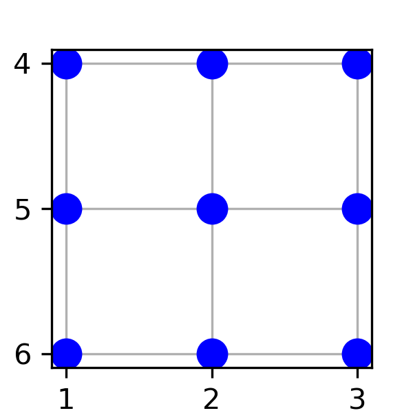
Fig. 5.12 Visualizing np.meshgrid(x, y) with x = np.array([1, 2, 3]) and y = np.array([4, 5, 6]).#
5.1.10.2. np.ix_: Selective Indexing#
Purpose:
np.ix_is a valuable function for constructing open mesh grids from multiple sequences. It facilitates the selection of specific elements within multi-dimensional arrays, making it efficient for a wide range of applications.Usage:
grid = np.ix_(x, y)
Output:
gridis a tuple containing 1D arrays, where each array represents one dimension of the grid. It contains all possible combinations of values from the input sequences.
Example:
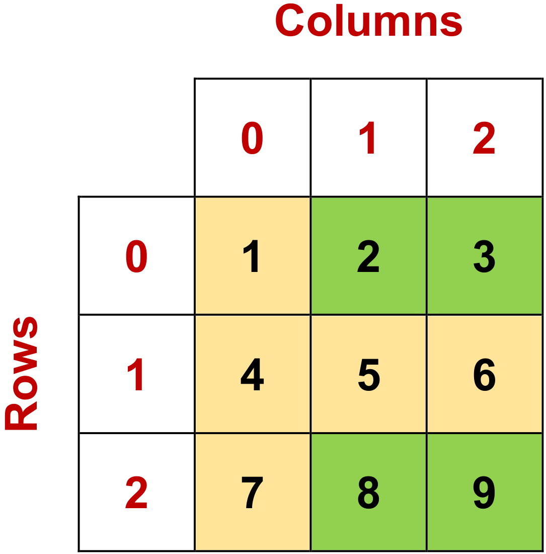
Fig. 5.13 Visualizing data[np.ix_(np.array([0, 2]), np.array([1, 2]))] with data = np.array([[1, 2, 3],[4, 5, 6],[7, 8, 9]]).#
# Create a 2D array for demonstration
data = np.array([[1, 2, 3],
                 [4, 5, 6],
                 [7, 8, 9]])

# Define indices for rows and columns using np.ix_
row_indices = np.array([0, 2])
col_indices = np.array([1, 2])

# Use np.ix_ to select specific elements
selected_elements = data[np.ix_(row_indices, col_indices)]

# selected_elements contains elements at (0,1), (0,2), (2,1), and (2,2)
print_bold("Selected Elements:")
pprint(selected_elements)
Selected Elements:
array([[2, 3],
       [8, 9]])
In this example, np.ix_ is used to create a grid of indices for rows and columns. The resulting selected_elements array contains elements at the specified row and column intersections, demonstrating the selective indexing capability of np.ix_.
These two NumPy functions, np.meshgrid and np.ix_, are fundamental tools that enable the creation of grids for visualization and efficient indexing for data manipulation. Understanding their usage is crucial for working effectively with multi-dimensional data in the NumPy library. The following sections will delve into practical applications and examples to showcase their versatility and utility.