Combining Datasets using Pandas

6.5. Combining Datasets using Pandas#

Within the Pandas library, merge, join, and concat are fundamental functions that hold pivotal significance in the process of combining and merging data from various DataFrames.

6.5.1. Pandas `merge`#

In Pandas, the merge function facilitates the merging of two DataFrames based on common columns or indices, resembling the behavior of SQL joins. By specifying the on parameter, you can identify the shared column(s) for merging. This function supports various types of joins, such as inner, left, right, and outer joins. To use merge, you simply follow this syntax [Pandas Developers, 2023]:

pd.merge(left, right, how='inner', on=None, left_on=None, right_on=None,
         left_index=False, right_index=False, sort=False, suffixes=('_x', '_y'),
         copy=True, indicator=False, validate=None)

Now, let’s explain each parameter:

left: The left DataFrame to be merged.
right: The right DataFrame to be merged.
how: The type of join to perform: 'inner', 'outer', 'left', 'right' or , 'cross'. Default is 'inner'.
on: Column(s) to join on. It can be a single column name or a list of column names.
left_on: Column(s) from the left DataFrame to use as join keys.
right_on: Column(s) from the right DataFrame to use as join keys.
left_index: If True, use the left DataFrame’s index as a join key.
right_index: If True, use the right DataFrame’s index as a join key.
sort: Sort the result DataFrame by the join keys.
suffixes: Suffixes to add to overlapping column names from both DataFrames.
copy: If True, creates copies of input data.
indicator: If True, adds a column to indicate the source of each row.
validate: Validates the merge keys: 'one_to_one', 'one_to_many', 'many_to_one', 'many_to_many'.

The merge() function is used to combine two or more DataFrames based on common columns or indices. The how parameter determines the type of join (inner, outer, left, right). The on, left_on, and right_on parameters specify which columns to use as keys. The left_index and right_index parameters indicate whether to use the indices for joining. The suffixes parameter is used to handle overlapping column names.

For a comprehensive understanding of the function, you may refer to the complete documentation available here.

These are the different types of merge operations that you can specify when combining dataframes using the merge() function in pandas [McKinney, 2022]:

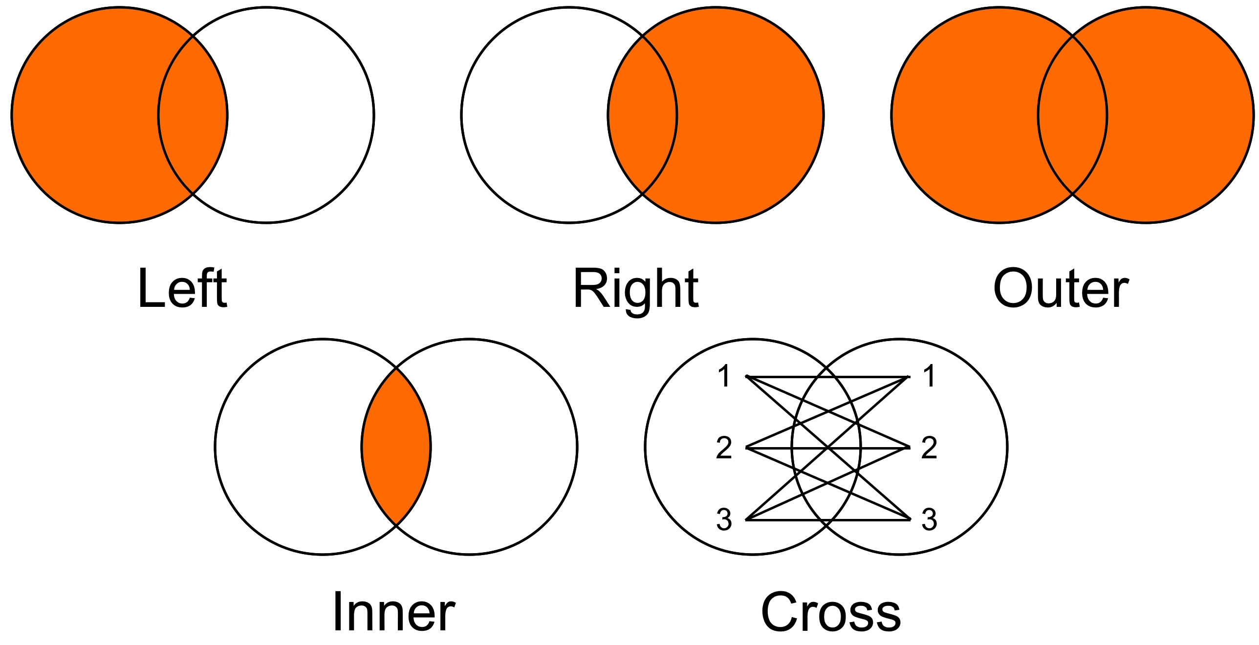
../_images/join_how.jpg — Fig. 6.18 Pandas `how` visualization.#

Inner Merge ('inner'):
- The inner merge returns only the rows where the keys (columns used for merging) exist in both dataframes.
- It effectively performs an intersection of the keys and retains only the common rows between the dataframes.

import pandas as pd

# Create two DataFrames
df1 = pd.DataFrame({'ID': [1, 2, 3], 'Name': ['Alice', 'Bob', 'Charlie']})
df2 = pd.DataFrame({'ID': [2, 3, 4], 'Age': [25, 30, 22]})

# Display the original DataFrames
print('df1:')
display(df1)
print('df1:')
display(df2)

# Perform an inner merge on 'ID' column
inner_merged = df1.merge(df2, on='ID', how='inner')

# Display the result of the inner merge
print('Mergerd df:')
display(inner_merged)

df1:

	ID	Name
0	1	Alice
1	2	Bob
2	3	Charlie

df1:

	ID	Age
0	2	25
1	3	30
2	4	22

Mergerd df:

	ID	Name	Age
0	2	Bob	25
1	3	Charlie	30

Outer Merge ('outer'):
- The outer merge returns all rows from both dataframes.
- If a key exists in one dataframe but not in the other, the missing values will be filled with NaN (or specified fill values) in the resulting dataframe.
- It effectively performs a union of the keys, including all rows from both dataframes.

# Display the original DataFrames
print('df1:')
display(df1)
print('df2:')
display(df2)

# Perform an outer merge on 'ID' and store the result in 'outer_merged'
outer_merged = df1.merge(df2, on='ID', how='outer')

# Display the result of the outer merge
print('Merged DataFrame:')
display(outer_merged)

df1:

	ID	Name
0	1	Alice
1	2	Bob
2	3	Charlie

df2:

	ID	Age
0	2	25
1	3	30
2	4	22

Merged DataFrame:

	ID	Name	Age
0	1	Alice	NaN
1	2	Bob	25.0
2	3	Charlie	30.0
3	4	NaN	22.0

Left Merge ('left'):
- The left merge returns all rows from the left dataframe and any matching rows from the right dataframe.
- If a key exists in the left dataframe but not in the right dataframe, the missing values in the right columns will be filled with NaN (or specified fill values) in the resulting dataframe.

# Display the original DataFrames
print('df1:')
display(df1)
print('df2:')
display(df2)

# Perform a left merge on 'ID' and store the result in 'left_merged'
left_merged = df1.merge(df2, on='ID', how='left')

# Display the result of the left merge
print('Merged DataFrame:')
display(left_merged)

df1:

	ID	Name
0	1	Alice
1	2	Bob
2	3	Charlie

df2:

	ID	Age
0	2	25
1	3	30
2	4	22

Merged DataFrame:

	ID	Name	Age
0	1	Alice	NaN
1	2	Bob	25.0
2	3	Charlie	30.0

Right Merge ('right'):
- The right merge is similar to the left merge but keeps all rows from the right dataframe and includes matching rows from the left dataframe.
- If a key exists in the right dataframe but not in the left dataframe, the missing values in the left columns will be filled with NaN (or specified fill values) in the resulting dataframe.

# Display the original DataFrames
print('df1:')
display(df1)
print('df2:')
display(df2)

# Perform a right merge on 'ID' and store the result in 'right_merged'
right_merged = df1.merge(df2, on='ID', how='right')

# Display the result of the right merge
print('Merged DataFrame:')
display(right_merged)

df1:

	ID	Name
0	1	Alice
1	2	Bob
2	3	Charlie

df2:

	ID	Age
0	2	25
1	3	30
2	4	22

Merged DataFrame:

	ID	Name	Age
0	2	Bob	25
1	3	Charlie	30
2	4	NaN	22

Cross Join ('cross'):
- The cross join (also known as a Cartesian product) combines every row from the first dataframe with every row from the second dataframe.
- It results in a dataframe with a size equal to the product of the number of rows in both input dataframes.
- Since it generates a large number of rows, it should be used with caution and only when explicitly needed

# Display the original DataFrames
print('df1:')
display(df1)
print('df2:')
display(df2)

# Perform a cross merge on 'ID' and store the result in 'cross_join'
cross_join = df1.merge(df2, how='cross', suffixes=('_df1', '_df2'))

# Display the result of the cross join
print('Merged DataFrame:')
display(cross_join)

df1:

	ID	Name
0	1	Alice
1	2	Bob
2	3	Charlie

df2:

	ID	Age
0	2	25
1	3	30
2	4	22

Merged DataFrame:

	ID_df1	Name	ID_df2	Age
0	1	Alice	2	25
1	1	Alice	3	30
2	1	Alice	4	22
3	2	Bob	2	25
4	2	Bob	3	30
5	2	Bob	4	22
6	3	Charlie	2	25
7	3	Charlie	3	30
8	3	Charlie	4	22

Here’s a quick summary of their behavior:

Merge Type	Description
`'inner'`	Retains rows with matching keys in both dataframes.
`'outer'`	Retains all rows, filling in missing values with `NaN` for non-matching keys.
`'left'`	Retains all rows from the left dataframe and matches them with rows from the right dataframe.
`'right'`	Retains all rows from the right dataframe and matches them with rows from the left dataframe.
`'cross'`	Generates a new dataframe with all possible combinations of rows from both dataframes.

6.5.1.1. Multi-Key Merging#

You can merge DataFrames on multiple columns by passing a list of column names to the on parameter.

merged_df = pd.merge(df1, df2, on=['key1', 'key2'])

Example:

import pandas as pd

# Create the first DataFrame
df1 = pd.DataFrame({'key1': ['A', 'B', 'C'],
                    'key2': ['X', 'Y', 'Z'],
                    'value': [10, 20, 30]
                    })

# Create the second DataFrame
df2 = pd.DataFrame({'key1': ['B', 'C', 'D'],
                    'key2': ['Y', 'Z', 'W'],
                    'value': [40, 50, 60]
                    })

# Display the first DataFrame
print('df1:')
display(df1)

# Display the second DataFrame
print('df2:')
display(df2)

# Merge the DataFrames based on the common keys 'key1' and 'key2'
merged_df = pd.merge(df1, df2, on=['key1', 'key2'])

# Display the merged DataFrame
print('Merged DataFrame:')
display(merged_df)

df1:

	key1	key2	value
0	A	X	10
1	B	Y	20
2	C	Z	30

df2:

	key1	key2	value
0	B	Y	40
1	C	Z	50
2	D	W	60

Merged DataFrame:

	key1	key2	value_x	value_y
0	B	Y	20	40
1	C	Z	30	50

The resulting DataFrame contains only the rows where ‘key1’ and ‘key2’ values were common between df1 and df2, and it shows the corresponding values from both DataFrames in separate columns (‘value_x’ and ‘value_y’).

6.5.1.2. Specifying Left and Right Prefixes#

When merging DataFrames with overlapping column names, you can specify prefixes to differentiate them.

merged_df = pd.merge(df1, df2, on='ID', suffixes=('_left', '_right'))

Example:

merged_df = pd.merge(df1, df2, on= ['key1', 'key2'], suffixes=('_left', '_right'))
display(merged_df)

	key1	key2	value_left	value_right
0	B	Y	20	40
1	C	Z	30	50

6.5.1.3. Merging on Index#

You can merge DataFrames based on their indices using the left_index and right_index parameters.

merged_df = pd.merge(df1, df2, left_index=True, right_index=True)

Example:

import pandas as pd

# Assuming df1 and df2 are already defined

# Set the index of df1 to 'key1'
df1.set_index('key1', inplace=True)

# Set the index of df2 to 'key1'
df2.set_index('key1', inplace=True)

# Merge the DataFrames based on their index (key1)
merged_df = pd.merge(df1, df2, left_index=True, right_index=True)

# Display the merged DataFrame
display(merged_df)

	key2_x	value_x	key2_y	value_y
key1
B	Y	20	Y	40
C	Z	30	Z	50

6.5.1.4. Merging and Filtering DataFrames in Pandas using merge() and query() (Optional Content)#

In Pandas, the merge() function is used to combine two or more DataFrames based on a common column or index. The query() function is used to filter rows from a DataFrame based on a given condition. Although you can use both functions separately, there might be scenarios where you want to merge DataFrames and then filter the result using a query [McKinney, 2022, Pandas Developers, 2023].

Example: Let’s assume you have two DataFrames, df1 and df2, and you want to merge them based on a common column, and then filter the merged result using a query condition.

import numpy as np
import pandas as pd

# Sample data for df1
df1 = pd.DataFrame({'ID': np.arange(0, 5),
                    'Value1': np.arange(0, 50, 10)
                    })
print('df1:')
display(df1)

# Sample data for df2
df2 = pd.DataFrame({'ID': np.arange(1, 8),
                    'Value2': np.arange(100, 800, 100)
                    })
print('df2:')
display(df2)

# Merge the two DataFrames on the 'ID' column using an inner join
merged_df = pd.merge(df1, df2, on='ID', how='inner')
print('Merged:')
display(merged_df)

# Filter the merged DataFrame using the query function
filtered_df = merged_df.query('Value1 > 15 and Value2 < 400')
print('Filtered:')
display(filtered_df)

df1:

	ID	Value1
0	0	0
1	1	10
2	2	20
3	3	30
4	4	40

df2:

	ID	Value2
0	1	100
1	2	200
2	3	300
3	4	400
4	5	500
5	6	600
6	7	700

Merged:

	ID	Value1	Value2
0	1	10	100
1	2	20	200
2	3	30	300
3	4	40	400

Filtered:

	ID	Value1	Value2
1	2	20	200
2	3	30	300

6.5.1.5. Semi-join and Anti-join (Optional Content)#

Semi-join and anti-join are concepts in relational database management systems that involve combining two tables based on a common column but with specific filtering conditions. These concepts are useful for filtering and retrieving rows that meet certain criteria while excluding others [Rioux, 2022, Pandas Developers, 2023].

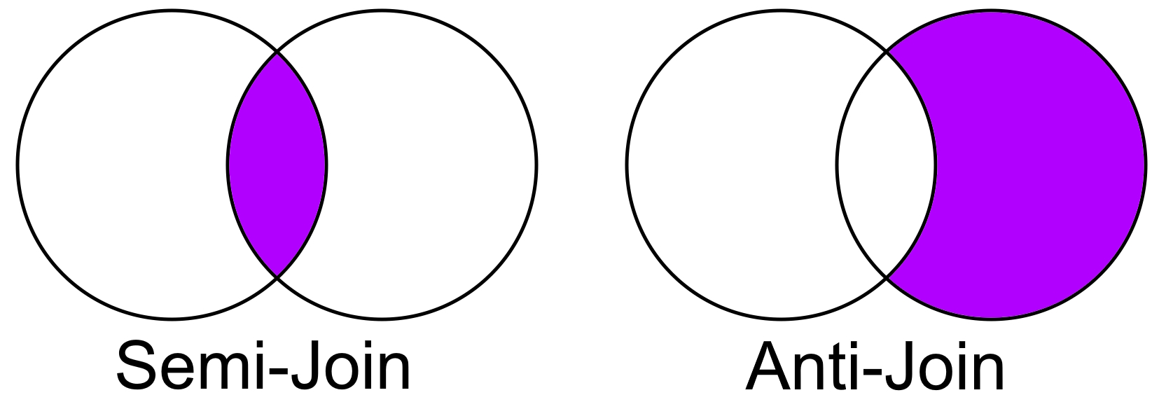
../_images/semi_join.jpg — Fig. 6.19 Semi join and Anti-join#

Semi-Join: A semi-join is a type of join operation that returns rows from the first table that match the condition in the second table. In other words, it selects rows from one table where there is a match in the other table based on a specified column. However, unlike a regular join, only the columns from the first table are included in the result [Rioux, 2022, Pandas Developers, 2023].
Anti-Join: An anti-join, also known as an anti-semi-join or difference join, is the opposite of a semi-join. It returns rows from the first table that do not have a match in the second table based on a specified column. Essentially, it filters out rows from the first table that meet a certain condition found in the second table [Rioux, 2022, Pandas Developers, 2023].

Remark

Semi-joins are typically used to filter data based on a condition present in another table.
Anti-joins are useful for finding records that are not present in another table or for excluding certain records that meet a certain criterion.

import pandas as pd

# Assuming df1 and df2 are already defined

# Print and display df1
print('df1:')
display(df1)

# Print and display df2
print('df2:')
display(df2)

# Semi-Join: Get rows from df1 that have matching IDs in df2
semi_join_result = df1[df1['ID'].isin(df2['ID'])]

# Anti-Join: Get rows from df1 that do not have matching IDs in df2
anti_join_result = df1[~df1['ID'].isin(df2['ID'])]

# Print Semi-Join Result
print("Semi-Join Result:")
display(semi_join_result)

# Print Anti-Join Result
print("Anti-Join Result:")
display(anti_join_result)

df1:

	ID	Value1
0	0	0
1	1	10
2	2	20
3	3	30
4	4	40

df2:

	ID	Value2
0	1	100
1	2	200
2	3	300
3	4	400
4	5	500
5	6	600
6	7	700

Semi-Join Result:

	ID	Value1
1	1	10
2	2	20
3	3	30
4	4	40

Anti-Join Result:

	ID	Value1
0	0	0

In SQL, you can use the LEFT JOIN (for semi-join) and NOT IN or NOT EXISTS (for anti-join) constructs to achieve these types of joins.

In Pandas, you can simulate these types of joins using various methods. For example, to perform a semi-join, you could use the merge() function with the desired how parameter and then select the columns you want. For an anti-join, you could use the merge() function with the indicator parameter and then filter out the matching rows [Rioux, 2022, Pandas Developers, 2023].

Here’s a simplified example in Pandas:

# Semi Join: Customers who have made orders
semi_join_df = df1.merge(df2[['ID']], on='ID', how='left', indicator=True)
semi_join_df = semi_join_df.query('_merge == "both"').drop('_merge', axis=1)
print("Semi-Join Result:")
display(semi_join_df)

# Anti Join: Customers who have not made orders
anti_join_df = df1.merge(df2[['ID']], on='ID', how='left', indicator=True)
anti_join_df = anti_join_df.query('_merge == "left_only"').drop('_merge', axis=1)
print("Anti-Join Result:")
display(anti_join_df)

Semi-Join Result:

	ID	Value1
1	1	10
2	2	20
3	3	30
4	4	40

Anti-Join Result:

	ID	Value1
0	0	0

Set Theory Notation for Joins:

Inner Join:
- Set Theory: A ∩ B
- Description: Includes rows that have matching values in both A and B.
Outer Join (Full Outer Join):
- Set Theory: A ∪ B
- Description: Includes all rows from both A and B, with missing values for non-matching rows.
Left Join:
- Set Theory: A ∪ (A ∩ B)
- Description: Includes all rows from A and only the matching rows from B.
Right Join:
- Set Theory: B ∪ (A ∩ B)
- Description: Includes all rows from B and only the matching rows from A.
Cross Join (Cartesian Join):
- Set Theory: A × B
- Description: Creates all possible combinations of rows from A and B.
Semi-Join (Left or Right):
- Set Theory: A ∩ B
- Description: Includes rows from one DataFrame (A or B) that have matching values in the other DataFrame.
Anti-Join:
- Set Theory: B - (A ∩ B)
- Description: Includes rows from B that do not have matching values in A.

Summary:

Join Type	Notation	Description
Inner Join	A ∩ B	Rows with matching values in both A and B
Outer Join	A ∪ B	All rows from both A and B, with missing values
Left Join	A ∪ (A ∩ B)	All rows from A, only matching rows from B
Right Join	B ∪ (A ∩ B)	All rows from B, only matching rows from A
Cross Join	A × B	All possible combinations of rows from A and B
Semi-Join	A ∩ B	Rows from one DataFrame (A or B) with matching values
Anti-Join	B - (A ∩ B)	Rows from B without matching values in A

This table summarizes the various types of joins using set theory notation and provides brief descriptions of each join operation.

6.5.1.6. Merge on Nearest Key (Optional Content)#

The pd.merge_asof() function in Pandas is used to perform a merge based on the nearest key, particularly for ordered data. It’s often used when you want to match records in two datasets based on a key column, but the values in the key column may not match exactly. Instead of requiring exact matches, this function allows you to match the nearest key values within a specified tolerance [McKinney and others, 2010, Pandas Developers, 2023].

Here’s the syntax of the pd.merge_asof() function:

pd.merge_asof(left, right, on, by, left_on, right_on, left_index, right_index, direction, tolerance)

left: The left DataFrame to merge.
right: The right DataFrame to merge.
on: The column name to use as the key for merging. It must be present in both DataFrames.
by: A list of columns to be used as additional keys for merging.
left_on, right_on: Columns from the left and right DataFrames to use as keys instead of the on parameter.
left_index, right_index: If True, use the index of the left or right DataFrame as a key.
direction: Specifies whether to search for the nearest key in ‘backward’ or ‘forward’ direction.
tolerance: The maximum allowable difference between key values for a successful match.

Here’s an explanation of the parameters using an example:

import pandas as pd

# Creating stock price and economic data DataFrames
stock_prices = pd.DataFrame({'timestamp': ['2023-01-01 09:00:00', '2023-01-01 09:15:00', '2023-01-01 09:30:00'],
                             'stock_symbol': ['AAPL', 'AAPL', 'AAPL'],
                             'price': [150.20, 152.40, 153.10]
                             })
print('Stock Prices:')
display(stock_prices)

economic_data = pd.DataFrame({'timestamp': ['2023-01-01 09:05:00', '2023-01-01 09:25:00', '2023-01-01 09:40:00'],
                              'indicator': ['GDP', 'Unemployment', 'Inflation'],
                              'value': [2.5, 4.8, 2.2]
                              })
print('Economic Data:')
display(economic_data)

# Converting timestamps to datetime format
stock_prices['timestamp'] = pd.to_datetime(stock_prices['timestamp'])
economic_data['timestamp'] = pd.to_datetime(economic_data['timestamp'])

# Merging based on the nearest key
merged_df = pd.merge_asof(stock_prices, economic_data, on='timestamp')

# Displaying the result
print('Merged DataFrame:')
display(merged_df)

Stock Prices:

	timestamp	stock_symbol	price
0	2023-01-01 09:00:00	AAPL	150.2
1	2023-01-01 09:15:00	AAPL	152.4
2	2023-01-01 09:30:00	AAPL	153.1

Economic Data:

	timestamp	indicator	value
0	2023-01-01 09:05:00	GDP	2.5
1	2023-01-01 09:25:00	Unemployment	4.8
2	2023-01-01 09:40:00	Inflation	2.2

Merged DataFrame:

	timestamp	stock_symbol	price	indicator	value
0	2023-01-01 09:00:00	AAPL	150.2	NaN	NaN
1	2023-01-01 09:15:00	AAPL	152.4	GDP	2.5
2	2023-01-01 09:30:00	AAPL	153.1	Unemployment	4.8

Remark

The choice between using pd.merge and pd.merge_asof depends on the specific use case and the desired merging behavior. Both methods are useful for merging datasets, but they have different purposes and are suited for different scenarios.

pd.merge is generally used for precise merges on exact match conditions, including merges on columns other than datetime. It provides options for different types of joins (e.g., inner, outer, left, right), and it requires an exact match on the specified merge column(s).

pd.merge_asof, on the other hand, is specifically designed for merging based on nearest key(s) with an optional tolerance. This method is particularly useful when you want to merge datasets based on datetime columns, and you want to match rows within a certain time range (tolerance) rather than requiring an exact match.

Here’s an example of when you might prefer to use pd.merge_asof:

import pandas as pd

# Sample DataFrames with datetime columns
data1 = {
    "datetime": ["2023-01-01", "2023-02-01", "2023-03-01", "2023-04-01"],
    "value1": [10, 20, 30, 40],
}
df1 = pd.DataFrame(data1)

data2 = {
    "datetime": ["2023-01-15", "2023-03-01", "2023-03-15"],
    "value2": [100, 200, 300],
}
df2 = pd.DataFrame(data2)

# Convert the 'datetime' column to datetime format
df1['datetime'] = pd.to_datetime(df1['datetime'])
df2['datetime'] = pd.to_datetime(df2['datetime'])

# Merge based on nearest datetime with a tolerance
merged_df = pd.merge_asof(df1, df2, on='datetime', tolerance=pd.Timedelta(days=15))

# Print the merged DataFrame
print(merged_df)

    datetime  value1  value2
2023-01-01      10     NaN
2023-02-01      20     NaN
2023-03-01      30   200.0
2023-04-01      40     NaN

In this code, pd.merge_asof is used to merge df1 and df2 based on the “datetime” column with a tolerance of 15 days. This means rows from df2 will be matched to the nearest row in df1 based on the datetime column, allowing for a difference of up to 15 days.

6.5.1.7. Categorical Merging#

If your data has categorical variables, you can use categorical merging for better performance.

df1['category_column'] = df1['category_column'].astype('category')
df2['category_column'] = df2['category_column'].astype('category')
merged_df = pd.merge(df1, df2, on='category_column')

Example:

import pandas as pd
import numpy as np
import time

# Generating example data
n = int(1e4)  # Number of rows
categories = ['A', 'B', 'C', 'D', 'E']
np.random.seed(42)
df1 = pd.DataFrame({
    'id': np.arange(n),
    'category_column': np.random.choice(categories, size=n)
})
df2 = pd.DataFrame({
    'category_column': np.random.choice(categories, size=n),
    'value': np.random.randint(1, 100, size=n)
})

# Regular merging (without categorical data type)
start_time = time.time()
regular_merged_df = pd.merge(df1, df2, on='category_column')
regular_merge_time = time.time() - start_time

# Converting the 'category_column' to categorical data type
df1['category_column'] = df1['category_column'].astype('category')
df2['category_column'] = df2['category_column'].astype('category')

# Categorical merging
start_time = time.time()
categorical_merged_df = pd.merge(df1, df2, on='category_column')
categorical_merge_time = time.time() - start_time

# Displaying results
print(f"Regular Merge Time: {regular_merge_time:.3f}")
print(f"Categorical Merge Time: {categorical_merge_time:.3f}")

Regular Merge Time: 0.486
Categorical Merge Time: 0.309

In this example, we generate two DataFrames, df1 and df2, with a categorical column ‘category_column’. We then compare the performance of regular merging versus categorical merging.

Categorical merging can offer better performance, especially when dealing with large datasets, because categorical data types use integer-based codes internally, reducing memory usage and speeding up comparison operations. As a result, merging operations involving categorical columns can be more efficient.

Remember that the actual performance gain will depend on various factors including the size of your dataset and the specific operations being performed. Always consider the benefits of categorical data types based on your use case.

These advanced merging techniques provide more flexibility and control over how you combine datasets using Pandas. Be sure to refer to the Pandas documentation for detailed information on these methods and their parameters: https://pandas.pydata.org/docs/reference/api/pandas.DataFrame.merge.html

6.5.2. Pandas `join`#

In pandas, the join() method is used to combine two DataFrame objects based on their index or on a key column. It is one of the methods for data alignment and merging in pandas. This operation can be compared to a database-style join. The basic syntax for the join() method is as follows [McKinney and others, 2010, Pandas Developers, 2023]:

result = left_dataframe.join(right_dataframe, how='inner')

Here, left_dataframe is the DataFrame to which you want to join another DataFrame (right_dataframe). The how parameter specifies the type of join to perform, and it can take the following values:

'inner': Performs an inner join, keeping only the rows that have matching keys in both DataFrames.
'outer': Performs an outer join, keeping all the rows from both DataFrames and filling in NaN values for missing keys.
'left': Performs a left join, keeping all the rows from the left DataFrame and filling in NaN values for missing keys in the right DataFrame.
'right': Performs a right join, keeping all the rows from the right DataFrame and filling in NaN values for missing keys in the left DataFrame.
'cross': “The cross merge method produces the Cartesian product of both data frames while maintaining the original order of the left keys.”

For a comprehensive description of the function, please refer to the official documentation here.

6.5.2.1. Basic Join Using Indices#

import pandas as pd

# Creating example DataFrames
df1 = pd.DataFrame({'A': [1, 2, 3], 'B': [4, 5, 6]}, index=['X', 'Y', 'Z'])
df2 = pd.DataFrame({'C': [7, 8, 9], 'D': [10, 11, 12]}, index=['X', 'Y', 'Z'])

# Title: Joining DataFrames Based on Indices

# Print the original DataFrames
print("Original df1:")
display(df1)

print("\nOriginal df2:")
display(df2)

# Joining based on indices
joined_df = df1.join(df2)

# Title: Displaying the Result

# Print the resulting joined DataFrame
print("\nJoined DataFrame (based on indices):")
display(joined_df)

Original df1:

	A	B
X	1	4
Y	2	5
Z	3	6

Original df2:

	C	D
X	7	10
Y	8	11
Z	9	12

Joined DataFrame (based on indices):

	A	B	C	D
X	1	4	7	10
Y	2	5	8	11
Z	3	6	9	12

The code demonstrates how the join() method can be used to combine two DataFrames using their indices, resulting in a new DataFrame where columns from both DataFrames are aligned based on the shared index labels. In this example, the resulting DataFrame will have columns ‘A’, ‘B’, ‘C’, and ‘D’.

6.5.2.2. Specifying Join Type and Suffixes#

In data manipulation with Pandas, specifying the join type and using custom suffixes can be essential when combining DataFrames.

Example:

import pandas as pd

# Creating example DataFrames
df1 = pd.DataFrame({'A': [1, 2, 3], 'B': [4, 5, 6]}, index=['X', 'Y', 'Z'])
df2 = pd.DataFrame({'B': [7, 8, 9], 'D': [10, 11, 12]}, index=['X', 'Y', 'Z'])

# Title: Joining DataFrames with Custom Suffixes

# Print the original DataFrames
print("Original df1:")
display(df1)

print("\nOriginal df2:")
display(df2)

# Performing an inner join with custom suffixes
joined_df_inner = df1.join(df2, how='inner', lsuffix='_left', rsuffix='_right')

# Title: Displaying the Result

# Print the resulting joined DataFrame
print("\nJoined DataFrame (inner join with custom suffixes):")
display(joined_df_inner)

Original df1:

	A	B
X	1	4
Y	2	5
Z	3	6

Original df2:

	B	D
X	7	10
Y	8	11
Z	9	12

Joined DataFrame (inner join with custom suffixes):

	A	B_left	B_right	D
X	1	4	7	10
Y	2	5	8	11
Z	3	6	9	12

This code snippet demonstrates how to use the Pandas library in Python to create, join, and display DataFrames:

df1 = pd.DataFrame({'A': [1, 2, 3], 'B': [4, 5, 6]}, index=['X', 'Y', 'Z']): Here, we create the first DataFrame, df1, with two columns ‘A’ and ‘B’, each containing a list of values. The index parameter assigns custom row indices ‘X’, ‘Y’, and ‘Z’ to the DataFrame.
df2 = pd.DataFrame({'B': [7, 8, 9], 'D': [10, 11, 12]}, index=['X', 'Y', 'Z']): Similarly, the second DataFrame, df2, is created with columns ‘B’ and ‘D’, along with the same custom row indices as df1.
joined_df_inner = df1.join(df2, how='inner', lsuffix='_left', rsuffix='_right'): This line performs an inner join operation between df1 and df2 using the join() method. The how='inner' argument specifies an inner join, which retains only the rows with matching indices in both DataFrames. Additionally, the lsuffix='_left' and rsuffix='_right' arguments are used to add custom suffixes to the columns with identical names in the two DataFrames to differentiate them.

6.5.2.3. Joining on a Column and Index#

In data manipulation with Pandas, it’s often necessary to combine DataFrames based on both columns and indices.

Example:

import pandas as pd

# Creating example DataFrames
students_df = pd.DataFrame({'student_id': [1, 2, 3],
                            'student_name': ['Alice', 'Bob', 'Charlie']})

scores_df = pd.DataFrame({'score': [85, 92, 78]},
                          index=[1, 2, 3])  # Index matches 'student_id'

# Title: Joining on a Column and Index

# Print the original DataFrames
print("Original students_df:")
display(students_df)

print("\nOriginal scores_df:")
display(scores_df)

# Joining students_df with scores_df on student_id and index
joined_df = students_df.join(scores_df, on='student_id')

# Title: Displaying the Result

# Print the resulting joined DataFrame
print("\nJoined DataFrame:")
display(joined_df)

Original students_df:

	student_id	student_name
0	1	Alice
1	2	Bob
2	3	Charlie

Original scores_df:

	score
1	85
2	92
3	78

Joined DataFrame:

	student_id	student_name	score
0	1	Alice	85
1	2	Bob	92
2	3	Charlie	78

The code demonstrates how to use the join() method to combine DataFrames on a specified column and index, effectively matching information from both DataFrames based on the shared ‘student_id’. The displayed output will show the combined information of student names and scores.

Example: The following Python code exemplifies the process of merging two Pandas DataFrames based on both a shared column and an index. These DataFrames pertain to city information, with a specific focus on cities located in the province of Alberta, Canada. It’s important to acknowledge that there might be discrepancies between the population figures presented in this example and the precise figures for the year 2023. For precise and up-to-date population statistics, it is advisable to consult official sources such as https://www.alberta.ca/population-statistics.

import pandas as pd

# Create a City DataFrame with city names and populations
cities_df = pd.DataFrame({'City_Name': ['Calgary', 'Edmonton', 'Lethbridge'],
                          'Population': [640000, 1544000, 106550]})
# Display the City DataFrame
display(cities_df)

# Create an Additional Details DataFrame with 'City_Name' as the index
details_df = pd.DataFrame({'City_Name': ['Calgary', 'Edmonton', 'Lethbridge'],
                           'Province': ['Alberta', 'Alberta', 'Alberta'],
                           'Area (km^2)': [825.3, 684.47, 127.2]})
# Set 'City_Name' as the index for the Additional Details DataFrame
details_df = details_df.set_index('City_Name')
# Display the Additional Details DataFrame
display(details_df)

# Join the City DataFrame with the Additional Details DataFrame using both the 'City_Name' column and index
joined_df = cities_df.join(details_df, on='City_Name')

# Display the resulting joined DataFrame
display(joined_df)

	City_Name	Population
0	Calgary	640000
1	Edmonton	1544000
2	Lethbridge	106550

	Province	Area (km^2)
City_Name
Calgary	Alberta	825.30
Edmonton	Alberta	684.47
Lethbridge	Alberta	127.20

	City_Name	Population	Province	Area (km^2)
0	Calgary	640000	Alberta	825.30
1	Edmonton	1544000	Alberta	684.47
2	Lethbridge	106550	Alberta	127.20

6.5.2.4. Joining with DataFrame and Series#

import pandas as pd

# Creating a DataFrame and a Series
df = pd.DataFrame({'A': [1, 2, 3], 'B': [4, 5, 6]})
series = pd.Series([10, 20, 30], name='C')

# Title: Joining a DataFrame with a Series

# Print the original DataFrame and Series
print("Original DataFrame (df):")
display(df)

print("\nOriginal Series (series):")
display(series)

# Joining the DataFrame with the Series
joined_df = df.join(series)

# Title: Displaying the Result

# Print the resulting joined DataFrame
print("\nJoined DataFrame:")
display(joined_df)

Original DataFrame (df):

	A	B
0	1	4
1	2	5
2	3	6

Original Series (series):

  10
  20
  30
Name: C, dtype: int64

Joined DataFrame:

	A	B	C
0	1	4	10
1	2	5	20
2	3	6	30

6.5.2.5. Joining with a MultiIndex DataFrame#

import pandas as pd

# Creating example DataFrames with MultiIndex
index = pd.MultiIndex.from_tuples([('X', 1), ('Y', 2), ('Z', 3)], names=['idx', 'value'])
df1 = pd.DataFrame({'A': [10, 20, 30]}, index=index)
print('df1')
display(df1)

df2 = pd.DataFrame({'B': [100, 200, 300]},
                   index=pd.MultiIndex.from_tuples([('X', 1), ('Y', 2), ('Z', 4)], names=['idx', 'value']))
print('df2')
display(df2)
# Joining df1 with df2 on the MultiIndex 'idx' and 'value'
joined_df = df1.join(df2, on=['idx', 'value'])

# Displaying the result
display(joined_df)

df1

		A
idx	value
X	1	10
Y	2	20
Z	3	30

df2

		B
idx	value
X	1	100
Y	2	200
Z	4	300

		A	B
idx	value
X	1	10	100.0
Y	2	20	200.0
Z	3	30	NaN

This example demonstrates how to use the join() method to combine DataFrames with MultiIndexes based on specific MultiIndex levels.

The join() method in Pandas is useful when working with indexed data and when you want a more concise way to combine DataFrames. It offers flexibility in terms of specifying join types, handling multi-index data, and broadcasting along different axes. Remember to consult the Pandas documentation for more information on the join() method and its parameters: https://pandas.pydata.org/docs/reference/api/pandas.DataFrame.join.html

6.5.3. Pandas `concat`#

In pandas, the concat() function is used to concatenate two or more DataFrames along a particular axis (either row-wise or column-wise). This allows you to combine multiple DataFrames into a single DataFrame. The concat() function is quite versatile and can handle different concatenation scenarios. The basic syntax for the concat() function is as follows [McKinney and others, 2010, Pandas Developers, 2023]:

result = pd.concat([df1, df2, ...], axis=0)

Here, df1, df2, etc., are the DataFrames you want to concatenate. The axis parameter specifies the axis along which the concatenation will be performed:

axis=0 (default): Concatenate along the rows (vertical concatenation).
axis=1: Concatenate along the columns (horizontal concatenation).

Example: Vertical Concatenation (Concatenate along rows)

import pandas as pd

# Sample DataFrames
data1 = {'A': [1, 2, 3], 'B': [4, 5, 6]}
data2 = {'A': [7, 8, 9], 'B': [10, 11, 12]}
df1 = pd.DataFrame(data1)
df2 = pd.DataFrame(data2)

# Concatenate vertically (along rows)
result_vertical = pd.concat([df1, df2], axis=0)

# Display the concatenated DataFrame
display(result_vertical)

	A	B
0	1	4
1	2	5
2	3	6
0	7	10
1	8	11
2	9	12

Example: Horizontal Concatenation (Concatenate along columns)

import pandas as pd

# Sample DataFrames
data1 = {'A': [1, 2, 3], 'B': [4, 5, 6]}
data2 = {'C': [7, 8, 9], 'D': [10, 11, 12]}
df1 = pd.DataFrame(data1)
df2 = pd.DataFrame(data2)

# Concatenate horizontally (along columns)
result_horizontal = pd.concat([df1, df2], axis=1)

# Display the concatenated DataFrame
display(result_horizontal)

	A	B	C	D
0	1	4	7	10
1	2	5	8	11
2	3	6	9	12

Note that when concatenating along a particular axis, the DataFrames should have compatible shapes along that axis (i.e., the number of rows for vertical concatenation and the number of columns for horizontal concatenation).

The concat() function also allows you to handle duplicate indices, specify whether to ignore the original indices, and more. For more complex concatenation scenarios, you can refer to the pandas documentation: https://pandas.pydata.org/pandas-docs/stable/reference/api/pandas.concat.html

Combining Datasets using Pandas

Contents

6.5. Combining Datasets using Pandas#

6.5.1. Pandas merge#

6.5.1.1. Multi-Key Merging#

6.5.1.2. Specifying Left and Right Prefixes#

6.5.1.3. Merging on Index#

6.5.1.4. Merging and Filtering DataFrames in Pandas using merge() and query() (Optional Content)#

6.5.1.5. Semi-join and Anti-join (Optional Content)#

6.5.1.6. Merge on Nearest Key (Optional Content)#

6.5.1.7. Categorical Merging#

6.5.2. Pandas join#

6.5.2.1. Basic Join Using Indices#

6.5.2.2. Specifying Join Type and Suffixes#

6.5.2.3. Joining on a Column and Index#

6.5.2.4. Joining with DataFrame and Series#

6.5.2.5. Joining with a MultiIndex DataFrame#

6.5.3. Pandas concat#

6.5.1. Pandas `merge`#

6.5.2. Pandas `join`#

6.5.3. Pandas `concat`#