9.2. An Introduction to Linear Regression#
Linear regression is a foundational statistical technique that’s used to establish a mathematical relationship between a dependent variable (often referred to as the response variable) and one or more independent variables (referred to as predictors). It operates under the assumption that this relationship can be approximated by a straight line.
The core formula for linear regression is expressed as follows:
Where:
\(Y\) represents the dependent variable (response).
\(X_1, X_2, \ldots, X_p\) are the independent variables (predictors).
\(\beta_0, \beta_1, \ldots, \beta_p\) are the coefficients (regression coefficients or model parameters).
\(\varepsilon\) denotes the error term, accounting for unexplained variability.
The objective of linear regression is to determine the coefficients \(\beta_0, \beta_1, \ldots, \beta_p\) in a manner that optimally fits the observed data. The prevalent approach to estimating these coefficients is the least-squares method, which minimizes the sum of squared residuals [James et al., 2023]:
Here:
\(y_i\) is the observed value of the dependent variable.
\(\hat{y}_i\) is the predicted value based on the model.
\(n\) is the number of data points.
The coefficient estimation process involves using a training dataset with known values of \(Y\) and \(X\). The aim is to find the \(\beta\) values that minimize the RSS. This is typically achieved using numerical optimization techniques.
After the coefficients are estimated, the linear regression model can be applied to make predictions for new data points. Given the values of the independent variables \(X_1, X_2, \ldots, X_p\), the predicted value of the dependent variable \(Y\) is calculated using this equation [James et al., 2023]:
where \(\hat{\beta_0}, \hat{\beta_1}, \ldots, \hat{\beta_p}\) denote estimated value for unknown coefficients \(\beta_0, \beta_1, \ldots, \beta_p\).
Linear regression accommodates both simple linear regression (with a single predictor) and multiple linear regression (involving multiple predictors). It’s extensively employed across diverse fields, including statistics, economics, social sciences, and machine learning, for tasks like prediction, forecasting, and understanding the relationships between variables.
Note
In this context, the hat symbol (ˆ) is employed to signify the estimated value for an unknown parameter or coefficient, or to represent the predicted value of the response.
9.2.1. Estimating Beta Coefficients in Linear Regression using Least Squares#
The estimation of beta coefficients in linear regression, also known as the model parameters or regression coefficients, is a key step in fitting the regression model to the data. The most commonly used method for estimating these coefficients is the least squares approach. The goal is to find the values of the coefficients that minimize the sum of squared residuals (RSS), which measures the discrepancy between the observed values and the values predicted by the model.
Here’s a step-by-step overview of how beta coefficients are estimated using the least squares method:
Formulate the Objective: The linear regression model is defined as:
(9.39)#\[\begin{equation} Y = \beta_0 + \beta_1 X_1 + \beta_2 X_2 + \ldots + \beta_p X_p + \varepsilon \end{equation}\]The goal is to find the values of \(\beta_0, \beta_1, \ldots, \beta_p\) that minimize the RSS:
(9.40)#\[\begin{equation} \text{RSS} = \sum_{i=0}^{n} (y_i - \hat{y}_i)^2 \end{equation}\]Where:
\(y_i\) is the observed value of the dependent variable.
\(\hat{y}_i\) is the predicted value of the dependent variable based on the model.
\(n\) is the number of data points.
Differentiate the RSS: Take the partial derivatives of the RSS with respect to each coefficient \(\beta_j\) (for \(j=0\) to \(p\)) and set them equal to zero. This step finds the values of the coefficients that minimize the RSS.
Solve the Equations: The equations obtained from differentiation are a set of linear equations in terms of the coefficients. You can solve these equations to obtain the estimated values of \(\beta_0, \beta_1, \ldots, \beta_p\).
Interpretation: Once the coefficients are estimated, you can interpret their values. Each coefficient \(\beta_j\) represents the change in the mean response for a one-unit change in the corresponding predictor \(X_j\), while holding all other predictors constant.
Assumptions: It’s important to note that linear regression makes certain assumptions about the data, such as linearity, independence of errors, constant variance of errors (homoscedasticity), and normality of errors. These assumptions should be checked to ensure the validity of the regression results.
Implementation: In practice, numerical optimization techniques are often used to solve the equations and estimate the coefficients, especially when dealing with complex models or large datasets. Software packages like Python’s
scikit-learn[Pedregosa et al., 2011, scikit-learn Developers, 2023],statsmodels[Seabold and Perktold, 2010], and others provide functions for performing linear regression and estimating the coefficients.
The resulting estimated coefficients represent the best-fitting linear relationship between the dependent variable and the independent variables in the least squares sense.
Key Assumptions for Linear Regression Validity and Consequences of Violations:
Linear regression rests upon a foundational set of assumptions that are pivotal for ensuring the model’s reliability and the accuracy of its estimates. These critical assumptions, as delineated in [Frost, 2020, James et al., 2023, Roback and Legler, 2021], encompass the following:
Linearity: The relationship between the dependent variable and the independent variables must adhere to a linear pattern. This assumption is vital to accurately capture the inherent relationships within the data. If violated, the model might misrepresent the true relationships, leading to inaccurate predictions and biased coefficient estimates.
Independence: The error terms (\(\varepsilon\)) must be independent of one another. This assumption guards against correlated errors, which could result in biased or inefficient estimates. Violations could cause the model to overstate its precision, leading to unreliable inferences.
Homoscedasticity: The variance of the error terms should remain consistent across all levels of the predictors. In simpler terms, the spread of residuals should exhibit uniformity, reflecting consistent variability throughout the dataset. Breach of this assumption could introduce heteroscedasticity, wherein the variability of errors differs across levels of predictors. This might undermine the accuracy of statistical tests and lead to imprecise confidence intervals.
Normality: The error terms should conform to a normal distribution with a mean of zero. This assumption is instrumental for valid statistical inference and hypothesis testing associated with linear regression. Deviations from normality might not have severe consequences if the sample size is sufficiently large. However, in smaller samples, violations could compromise the accuracy of statistical tests.
No Perfect Multicollinearity: The independent variables should not exhibit perfect multicollinearity, implying they should not be perfectly correlated with one another. Substantial multicollinearity can render the interpretation of individual predictor effects challenging and inflate the standard errors of coefficient estimates. This can make the model sensitive to small changes in data and lead to instability in the estimates.
Ensuring the fulfillment of these assumptions is paramount, as deviations can undermine the reliability and precision of the linear regression model’s results. It is imperative to scrutinize these assumptions before drawing conclusions from the model’s outcomes. Various diagnostic techniques, such as residual plots and statistical tests, can be employed to evaluate the soundness of these assumptions. If violations are identified, corrective measures like transformation of variables or employing more sophisticated modeling techniques might be necessary to mitigate their impact and enhance the validity of the model’s inferences.
Definition - Multicollinearity
Multicollinearity refers to a situation in which two or more independent variables in a regression model are highly correlated with each other. In other words, multicollinearity occurs when there is a strong linear relationship between two or more predictor variables.
9.2.2. Simple Linear Regression: Modeling a Single Variable Relationship#
Simple linear regression is a fundamental statistical technique that focuses on modeling the relationship between two variables: a dependent variable (often referred to as the response variable) and a single independent variable (commonly known as the predictor). This approach operates under the assumption of a linear relationship, implying that the connection between these variables can be approximated by a straight line.
The core equation for simple linear regression, as described in [James et al., 2023], is expressed as follows:
Where:
\(Y\) represents the dependent variable (response).
\(X\) is the independent variable (predictor).
\(\beta_0\) denotes the intercept, signifying the value of \(Y\) when \(X\) equals zero.
\(\beta_1\) represents the slope, indicating the change in \(Y\) for a one-unit change in \(X\).
\(\varepsilon\) is the error term, accounting for the unexplained variability within the model.
The objective of simple linear regression is to estimate the coefficients \(\beta_0\) and \(\beta_1\) in a manner that the line best fits the observed data. The widely-used method for estimating these coefficients is the least-squares approach, which minimizes the sum of squared residuals:
Here:
\(y_i\) is the observed value of the dependent variable (\(Y\)) for the \(i\)th data point.
\(\hat{y}_i\) is the predicted value of the dependent variable (\(Y\)) for the \(i\)th data point based on the model.
\(n\) is the number of data points.
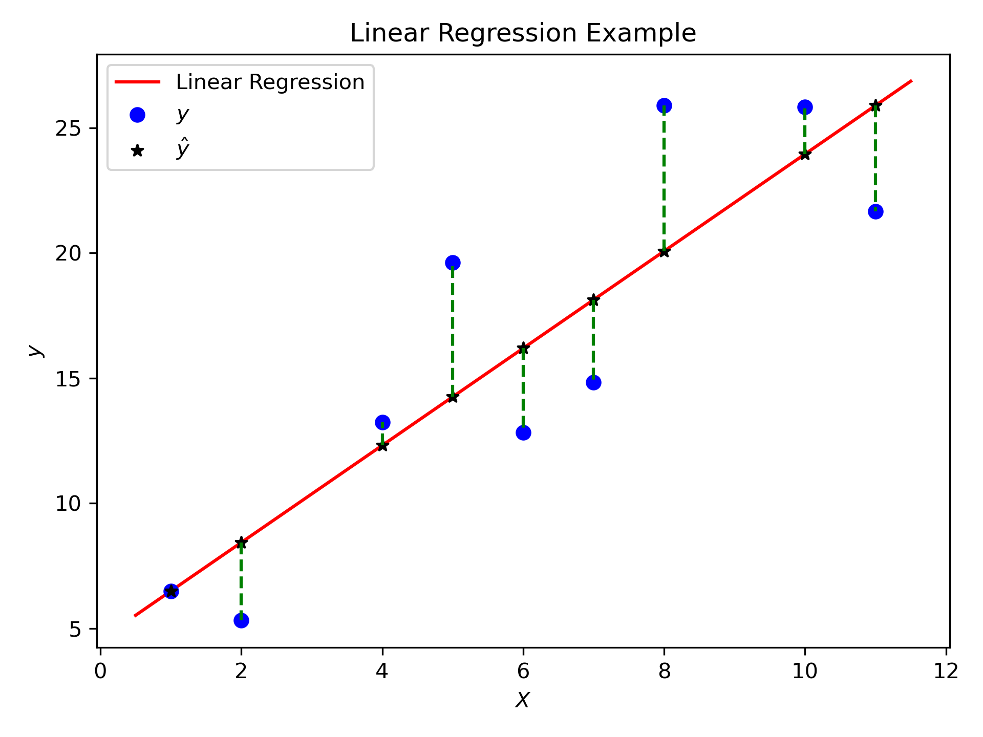
Fig. 9.4 The aggregate of the dashed green lines is elucidated as \(\text{RSS} = \sum_{i=0}^{n} (y_i - \hat{y}_i)^2\).#
Once the coefficients \(\beta_0\) and \(\beta_1\) are estimated, the simple linear regression model can be represented as:
where \(\hat{\beta_0}\) and \(\hat{\beta_1}\) denote estimated value for unknown coefficients \(\beta_0\) and \(\beta_1\).
This line serves as the best linear fit to the data and is utilized for making predictions regarding new data points. Given the value of the independent variable (\(X\)) for a new data point, the equation enables us to calculate the predicted value of the dependent variable (\(Y\)).
Simple linear regression finds broad applications across diverse fields, including economics, finance, social sciences, and engineering. It is particularly effective when a clear linear relationship exists between the two variables, enabling predictions and understanding the impact of the independent variable on the dependent variable, as highlighted in [James et al., 2023].
Nevertheless, interpreting the results of a simple linear regression analysis demands careful consideration. Factors such as goodness of fit (e.g., R-squared), statistical significance of the coefficients, and the validity of assumptions (e.g., linearity, independence of errors, normality of errors) should be taken into account to draw meaningful conclusions from the model. Furthermore, it’s essential to recognize that simple linear regression may not be suitable if the relationship between variables is nonlinear or if multiple predictors influence the dependent variable. In such cases, other approaches, such as multiple linear regression or more complex regression models, may be more appropriate, as discussed in [James et al., 2023].
9.2.2.1. Finding the intercept and the slope#
Finding the values of the coefficients \(\beta_0\) (the intercept) and \(\beta_1\) (the slope) in simple linear regression involves minimizing the sum of squared residuals (RSS). The RSS represents the difference between the observed values (\(y_i\)) and the predicted values (\(\hat{y}_i\)) based on the linear regression model for each data point. Mathematically, the objective is to find \(\beta_0\) and \(\beta_1\) that minimize the following expression:
Here’s a step-by-step mathematical derivation for finding \(\beta_0\) and \(\beta_1\):
Define the Linear Regression Model: Start with the basic linear regression equation:
Calculate the Predicted Values: The predicted value of \(Y\) (\(\hat{y}\)) for each data point is given by:
Define the Residuals: The residuals (\(e_i\)) are the differences between the observed values and the predicted values:
Formulate the Objective Function: The goal is to minimize the sum of squared residuals:
Find the Partial Derivatives: Compute the partial derivatives of the RSS with respect to \(\beta_0\) and \(\beta_1\):
Set the Derivatives to Zero and Solve: Set the partial derivatives to zero and solve the resulting system of equations for \(\beta_0\) and \(\beta_1\):
it follows that
The above linear system can be expressed in the following matrix form,
Once the optimal values of \(\beta_0\) and \(\beta_1\) are found, the simple linear regression model is defined as:
Where:
\(\hat{\beta_0}\) is the estimated intercept.
\(\hat{\beta_1}\) is the estimated slope.
This model represents the best-fit line that minimizes the sum of squared residuals and can be used for making predictions and understanding the relationship between the variables.
9.2.2.2. Finding the intercept and the slope (Vector Format)#
Given:
\( X \): The matrix of predictor variables (including an additional column of ones for the intercept).
\( y \): The vector of response variable values.
\( \beta \): The vector of coefficients (\(\beta_0\) and \(\beta_1\)).
Define the Linear Regression Model:
The linear regression model can be represented in matrix form as:
Where:
\( y \) is the vector of observed response values.
\( X \) is the matrix of predictor variables (including an additional column of ones for the intercept).
\( \beta \) is the vector of coefficients (\(\beta_0\) and \(\beta_1\)).
\( \varepsilon \) is the vector of error terms.
Calculate the Predicted Values:
The predicted values of \( y \) (\(\hat{y}\)) can be calculated as:
Define the Residuals:
The residuals can be defined as the difference between the observed values \( y \) and the predicted values \( \hat{y} \):
Formulate the Objective Function (Sum of Squared Residuals):
The objective is to minimize the sum of squared residuals:
Find the Optimal Coefficients:
The optimal coefficients \( \beta \), which we show it with \( \hat{\beta} \), can be found by minimizing the RSS:
Where:
\( X^T \) is the transpose of the matrix \( X \).
\( (X^T X)^{-1} \) is the inverse of the matrix \( X^T X \).
\( X^T y \) is the matrix-vector multiplication between \( X^T \) and \( y \).
Use the Optimal Coefficients for Prediction:
Once you have the optimal coefficients \( \hat{\beta} \), you can use them to predict new values of \( y \) based on new values of \( X \):
Where \( X_{\text{new}} \) is the matrix of new predictor variables.
Note
Let’s delve into the mathematical details of how we obtain the coefficient vector \( \hat{\beta} \) in linear regression. We’ll use matrix algebra to explain this process step by step.
Starting from the objective function to minimize the sum of squared residuals (RSS):
We can expand this expression and rewrite it as:
Now, let’s differentiate RSS with respect to \( \beta \) to find the minimum (i.e., where the gradient is zero). We use calculus to find the minimum point:
Therefore,
Setting this derivative equal to zero:
Now, we want to isolate \( \hat{\beta} \), so we’ll solve for it:
Now, we’ll distribute \( X^T \) and simplify:
To solve for \( \hat{\beta} \), we can isolate it on one side:
Now, to find \( \hat{\beta} \), we need to multiply both sides by the inverse of \( X^TX \):
So, \( \hat{\beta} \) is obtained by multiplying the inverse of the matrix \( X^TX \) with the product of \( X^T \) and \( y \).
9.2.2.3. The Hat matrix (Optional Content)#
Definition: The hat matrix, a fundamental tool in regression analysis and analysis of variance, serves as the bridge between observed values and estimations derived through the least squares method. In the context of linear regression represented in matrix form, if we denote \( \hat{y} \) as the vector comprising estimations calculated from the least squares parameters and \( y \) as a vector containing observations pertaining to the dependent variable, the relationship can be succinctly expressed as \( \hat{y} = Hy \), where \( H \) is the hat matrix responsible for transforming \( y \) into \( \hat{y}\) [Dodge, 2008].
(9.70)#\[\begin{equation} \hat{y} = X \beta = \underbrace{X(X^TX)^{-1}X^T}_{\text{Consider this part as }H}y \end{equation}\]Definition - Hat matrix
The Hat matrix, often denoted as \(H\), is a key concept in linear regression analysis. It plays a crucial role in understanding the influence of each observation on the fitted values of the regression model. The Hat matrix helps identify potential outliers, high-leverage points, and observations that have a significant impact on the model’s estimates [Cardinali, 2013, Meloun and Militký, 2011].
The Hat matrix is a projection matrix that maps the response variable values \(y\) to the predicted values \(\hat{y}\) obtained from the linear regression model. It is defined as [Cardinali, 2013, Meloun and Militký, 2011]:
(9.71)#\[\begin{equation} H = X(X^TX)^{-1}X^T \end{equation}\]Where:
\(X\) is the design matrix containing predictor variables (including a constant term for the intercept).
\(X^T\) is the transpose of \(X\).
\(X^TX\) is the matrix product of the transpose of \(X\) and \(X\).
\((X^TX)^{-1}\) is the inverse of the matrix \(X^TX\).
Diagonal Elements: The diagonal elements of the Hat matrix, denoted as \(h_{ii}\), represent the leverage of each observation \(i\). Leverage quantifies how much influence an observation has on the fitted values. Each \(h_{ii}\) value is calculated as:
(9.72)#\[\begin{equation} h_{ii} = (H)_{ii} = x_{i}^T (X^TX)^{-1}x_{i} \end{equation}\]Where:
\(x_{i}\) is the \(i\)-th row of the design matrix \(X\).
\((X^TX)^{-1}\) is the inverse of the matrix \(X^TX\).
Properties:
The diagonal elements of the Hat matrix range from \(0\) to \(1\). They indicate how much an observation’s predictor variables differ from the average values.
The average of the diagonal elements is [Dodge, 2008]
\[\begin{align*} \sum _{i=1}^{n}h_{ii} &= \operatorname {Tr} (\mathbf {H} )=\operatorname {Tr} \left(\mathbf {X} \left(\mathbf {X} ^{\top }\mathbf {X} \right)^{-1}\mathbf {X} ^{\top }\right)=\operatorname {Tr} \left(\mathbf {X} ^{\top }\mathbf {X} \left(\mathbf {X} ^{\top }\mathbf {X} \right)^{-1}\right)=\operatorname {Tr} (\mathbf {I} _{p})=p,\\ \bar {h} &= \dfrac {1}{n}\sum _{i=1}^{n}h_{ii}=\dfrac {p}{n}, \end{align*}\]where \(p\) refers to the number of predictor variables (also known as features or independent variables) in your regression model and \(n\) refers to the number of observations or data points in your dataset. This average represents the expected leverage of an observation.
Interpretation: High leverage points are observations with \(h_{ii}\) values close to 1, indicating that their predictor variable values are far from the mean. These points can significantly affect the fitted values and regression coefficients.
Influence Measures:
Leverage values help identify high-leverage points that may be potential outliers or influential observations.
Combined with the residuals, leverage values are used to calculate influence measures like Cook’s distance, which considers both leverage and residual information to assess the impact of an observation on the regression results.
Outliers and Model Assumptions:
Observations with high leverage values might not necessarily be outliers but could indicate extreme predictor variable values.
When checking assumptions of linear regression, examining high-leverage points can help detect deviations from linearity, normality, and constant variance assumptions.
Some statisticians consider \(x_{i}\) as an outlier if \({\displaystyle h_{ii}>2{\dfrac {p}{n}}}\).
Some other statisticians consider \(x_{i}\) as an outlier if \({\displaystyle h_{ii}>3{\dfrac {p}{n}}}\) [Cardinali, 2013].
Definition - Cook’s distance
Cook’s distance is a statistical measure that serves as a tool to identify outliers and influential observations in the context of regression analysis. It quantifies how much the fitted values of the response variable change when a specific observation is removed from the dataset. Cook’s distance is particularly helpful for detecting outliers in the predictor variables (X values) and assessing the impact of individual observations on the fitted response values. Observations with Cook’s distance exceeding three times the mean Cook’s distance might indicate potential outliers [Cardinali, 2013, Meloun and Militký, 2011, MATLAB Developers, 2023].
Definition
Each element of Cook’s distance (\(D\)) signifies the normalized alteration in the fitted response values due to the exclusion of a particular observation. The Cook’s distance for observation \(i\) is defined as [Cook, 2000, MATLAB Developers, 2023]:
Where:
\( n \) is the total number of observations.
\( p \) is the number of coefficients in the regression model.
\( \text{MSE} \) represents the mean squared error of the regression model.
\( \hat{y}_j \) is the fitted response value for the \(j\)th observation.
\( \hat{y}_{j(i)} \) is the fitted response value for the \(j\)th observation when observation \(i\) is omitted.
Algebraic Equivalent
Cook’s distance can also be expressed algebraically as follows [Cook, 2000, Kutner et al., 2004, MATLAB Developers, 2023]:
Where:
\( r_i \) is the residual for the \(i\)th observation.
\( h_{ii} \) is the leverage value for the \(i\)th observation.
In both forms, Cook’s distance reflects the combined effect of the squared differences in fitted response values after removing the \(i\)th observation, normalized by the model’s complexity (\(p\)) and the mean squared error. Additionally, the leverage value \(h_{ii}\) accounts for the influence of the \(i\)th observation’s predictor values.
High values of Cook’s distance indicate that the \(i\)-th observation has a substantial impact on the regression results and should be investigated further for potential influence or outliers. The leverage term (\(h_{ii}\)) provides insight into how much the \(i\)-th observation’s predictor values deviate from the average predictor values, contributing to its potential influence.
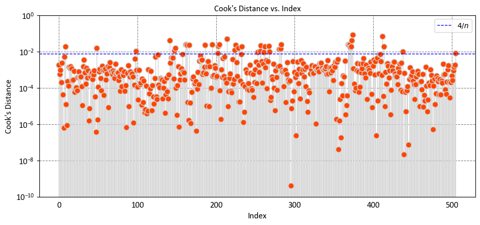
Interpreting Cook’s distance:
A larger Cook’s distance indicates that the corresponding data point has a significant impact on the regression model’s coefficients.
A small Cook’s distance suggests that the data point has less influence on the model.
The rule of thumb suggests that if the Cook’s distance for a specific data point exceeds 4/n, that data point is considered influential [RPubs by RStudio, 2023]. In general,
In other words, if the influence of a data point is relatively large, meaning it significantly affects the regression model’s coefficients and predictions, it might warrant closer examination.
However, it’s important to note that this rule of thumb is just a guideline, and the actual threshold value can vary depending on the context and the specific analysis. Additionally, the decision to consider a data point as influential should be made in conjunction with other diagnostic tools, domain knowledge, and the goals of the analysis.
To compute these values, you typically use the matrix algebra operations available in numerical libraries, as shown in your initial code. Here’s a step-by-step breakdown of the calculation for a single observation \( i \):
Retrieve the \( i \)-th row of the design matrix \( X \), denoted as \( x_{i} \).
Compute the matrix product \( X^TX \).
Compute the inverse of \( X^TX \).
Calculate the product \( x_{i}^T (X^TX)^{-1}x_{i} \) to obtain the leverage \( h_{ii} \).
These leverage values provide information about how influential each observation is on the fitted values and regression coefficients. High leverage points could potentially be outliers or observations with extreme predictor values that have a substantial impact on the model.
9.2.3. Example: Boston House-Price Data#
Example. To illustrate these concepts, we will employ the Boston Housing dataset. Widely utilized in machine learning and data science, Scikit-learn offers a range of tools for analysis. The Boston Housing dataset is a staple in regression analysis and can be accessed from the link: http://lib.stat.cmu.edu/datasets/boston. This dataset contains information about various features related to housing prices in different neighborhoods in Boston.
For our purposes, we will focus exclusively on three variables: LSTAT, and MEDV.
Variable |
Description |
|---|---|
LSTAT |
% lower status of the population |
MEDV |
Median value of owner-occupied homes in $1000’s |
import numpy as np
import pandas as pd

_url = "http://lib.stat.cmu.edu/datasets/boston"
columns = 12 *['_'] + ['LSTAT', 'MEDV']

Boston = pd.read_csv(filepath_or_buffer= _url, delim_whitespace=True, skiprows=21,
                 header=None)

#Flatten all the values into a single long list and remove the nulls
values_w_nulls = Boston.values.flatten()
all_values = values_w_nulls[~np.isnan(values_w_nulls)]

#Reshape the values to have 14 columns and make a new df out of them
Boston = pd.DataFrame(data = all_values.reshape(-1, len(columns)),
                      columns = columns)
Boston = Boston.drop(columns=['_'])
display(Boston)
| LSTAT | MEDV | |
|---|---|---|
| 0 | 4.98 | 24.0 |
| 1 | 9.14 | 21.6 |
| 2 | 4.03 | 34.7 |
| 3 | 2.94 | 33.4 |
| 4 | 5.33 | 36.2 |
| ... | ... | ... |
| 501 | 9.67 | 22.4 |
| 502 | 9.08 | 20.6 |
| 503 | 5.64 | 23.9 |
| 504 | 6.48 | 22.0 |
| 505 | 7.88 | 11.9 |
506 rows × 2 columns
To start, we will fit a simple linear regression model using the sm.OLS() function from statsmodels library. In this model, our response variable will be medv, and lstat will be the single predictor.
9.2.3.1. Loading the Data#
You have the Boston Housing dataset loaded, which contains variables like LSTAT (predictor) and MEDV (response).
# Select predictor and response variables
X = Boston['LSTAT'].values
y = Boston['MEDV'].values
9.2.3.2. Creating the Design Matrix#
After selecting the LSTAT variable as the predictor, you add a constant term to create the design matrix X.
Here, \( n \) is the number of observations in the dataset.
# Add a column of ones to the predictor matrix for the intercept term
X_with_intercept = np.column_stack((np.ones(len(X)), X))
print(X_with_intercept)
[[1.   4.98]
 [1.   9.14]
 [1.   4.03]
 ...
 [1.   5.64]
 [1.   6.48]
 [1.   7.88]]
9.2.3.3. Fitting the Linear Regression Model#
We fit the simple linear regression model: \( y = \beta_0 + \beta_1 \cdot \text{LSTAT} \), where \( y \) is the response variable MEDV and \(\text{LSTAT}\) is the predictor variable.
import warnings
warnings.simplefilter(action='ignore', category=FutureWarning)
import matplotlib.pyplot as plt
import numpy as np
plt.style.use('../mystyle.mplstyle')

def my_linear_regression(X, y):
    """
    Perform linear regression and return model coefficients, predicted values, and residuals.

    Parameters:
    X (numpy.ndarray): Input feature matrix with shape (n, p).
    y (numpy.ndarray): Target vector with shape (n,).

    Returns:
    float: Intercept of the linear regression model.
    numpy.ndarray: Array of slope coefficients for each feature.
    numpy.ndarray: Array of predicted values.
    numpy.ndarray: Array of residuals.
    """

    # Calculate the coefficients using the normal equation
    coeff_matrix = np.linalg.inv(X.T @ X) @ (X.T @ y)

    # Extract coefficients
    intercept, slope = coeff_matrix

    # Calculate the predicted values
    y_pred = X @ coeff_matrix

    # Calculate the residuals
    residuals = y - y_pred

    return intercept, slope, y_pred, residuals

intercept, slope, y_pred, residuals = my_linear_regression(X_with_intercept, y)

fig, ax = plt.subplots(1, 2, figsize=(9.5, 4.5), sharey = False)
ax = ax.ravel()
# regplot
_ = ax[0].scatter(x = X, y = y, fc= 'SkyBlue', ec = 'k', s = 50, label='Original Data')
_ = ax[0].set(xlabel = 'LSTAT', ylabel = 'MEDV',
              xlim = [-10, 50], ylim = [0, 60], title = 'Linear Regression')
xlim = ax[0].get_xlim()
ylim = [slope * xlim[0] + intercept, slope * xlim[1] + intercept]
_ = ax[0].plot(xlim, ylim, linestyle = 'dashed', color = 'red', lw = 3, label='Fitted Line')
_ = ax[0].legend()

# residuals
_ = ax[1].scatter(y_pred, residuals, fc='none', ec = 'DarkRed', s = 50)
_ = ax[1].axhline(0, c='k', ls='--')
_ = ax[1].set(aspect = 'auto',
              xlabel = 'Fitted value',
              ylabel = 'Residual',
              xlim = [0, 40], ylim = [-20, 30], title = 'Residuals for Linear Regression')
plt.tight_layout()

# Print the coefficients
print(f'Intercept: {intercept:.8f}')
print(f'Slope: {slope:.8f}')
Intercept: 34.55384088
Slope: -0.95004935
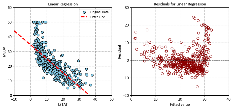
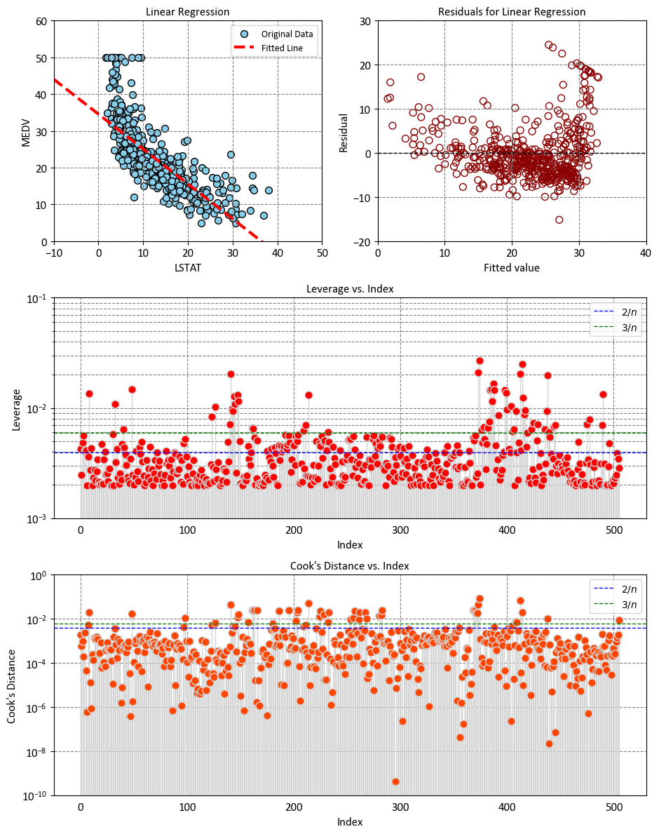
Left Plot: The plot shows that there is a negative linear relationship between LSTAT and MEDV, which means that as the percentage of lower status of the population increases, the median value of owner-occupied homes decreases. The plot also shows that the linear regression model fits the data reasonably well, as most of the points are close to the fitted line. However, there are some outliers and some curvature in the data, which indicate that the linear model may not capture all the features of the data. The plot can help us understand how LSTAT affects MEDV, and how well the linear regression model can predict MEDV based on LSTAT.
Right Plot: This plot shows the relationship between the fitted values and the residuals of a linear regression model. The fitted values are the predicted values of the response variable based on the predictor variable, and the residuals are the differences between the observed values and the predicted values. A residual plot can help you check the assumptions of a linear regression model, such as linearity, homoskedasticity, and normality of errors.
Remark
A plot of fitted values vs. residuals is a fundamental diagnostic tool in regression analysis. It visually represents the relationship between the predicted values (fitted values) and the corresponding residuals. This plot serves to assess the assumptions and model performance in regression analysis.
In this plot, the x-axis typically displays the fitted values obtained from the regression model, while the y-axis represents the residuals, which are the differences between the observed data points and the corresponding predicted values. By examining this plot, researchers can discern several key aspects [McPherson, 2001]:
Linearity: A random scatter of residuals around the horizontal axis indicates that the assumption of linearity is met. If a pattern is discernible (e.g., a curve or funnel shape), it suggests potential issues with linearity.
Homoscedasticity: The spread of residuals should remain roughly constant across the range of fitted values. A fan-shaped or widening pattern could indicate heteroscedasticity, where the variance of errors is not constant.
Independence of Errors: Ideally, there should be no discernible pattern or correlation among the residuals in the plot. Any systematic trends or clusters in the residuals may suggest omitted variables or autocorrelation.
Outliers and Influential Points: Outliers, which are data points with unusually large residuals, can be identified in this plot. Additionally, influential observations that significantly impact the model can be detected.
A plot of fitted values vs. residuals aids in assessing the validity of regression assumptions and the overall quality of the model fit. Researchers use this diagnostic tool to identify potential issues, guide model refinement, and ensure that the model’s predictions are reliable.
9.2.3.4. Calculating Hat Matrix Diagonal Values (Leverages) - (Optional Content)#
The Hat matrix \( H \) is calculated as \( H = X(X^TX)^{-1}X^T \). However, to compute leverage, you need the diagonal elements of \( H \), which is given by:
Here’s how you compute \( h_{ii} \) for each observation:
For the \( i \)-th observation, you take the \( i \)-th row of the design matrix \( X \), denoted as \( x_{i} \).
You calculate \( (X^TX)^{-1} \) as well.
Then, you perform the multiplication \( x_{i}^T (X^TX)^{-1}x_{i} \) to get the leverage \( h_{ii} \) for that observation.
This process is repeated for each observation, resulting in an array of leverage values.
In mathematical terms, for each observation \( i \), you compute the leverage \( h_{ii} \) using:
Where:
\( x_{i} \) is the \( i \)-th row of the design matrix \( X \).
\( (X^TX)^{-1} \) is the inverse of the matrix \( X^TX \).
In code, this is implemented as follows:
def leverage (X):
    XTX_inverse = np.linalg.inv(np.dot(X.T, X))
    leverage_values = np.diagonal(np.dot(np.dot(X, XTX_inverse), X.T))
    return leverage_values
Now, the leverage_values array contains the leverage values (Hat matrix diagonal values) for each observation. These values indicate how much influence each observation has on the fitted values of the regression model.
leverage_values = leverage(X_with_intercept)

fig, ax = plt.subplots(1, 1, figsize=(9.5, 4.5))
n = X.shape[0]
markerline, stemlines, baseline = ax.stem(np.arange(n), leverage_values,
                                          linefmt='lightgrey', markerfmt='o')
_ = markerline.set_markerfacecolor('red')
_ = ax.set(aspect = 'auto', xlabel = 'Index', ylabel = 'Leverage', title = 'Leverage vs. Index',
           yscale = 'log',  ylim = [1e-3, 1e-1])
_ = ax.tick_params(axis='x', which='both', bottom=False, top=False)  # Remove x-axis ticks
_ = ax.axhline(y=np.mean(2/n), color='blue', linestyle='--', label= r'$2/n$')
_ = ax.axhline(y=np.mean(3/n), color='green', linestyle='--', label= r'$3/n$')
_ = ax.legend()
# Fig setting
plt.tight_layout()
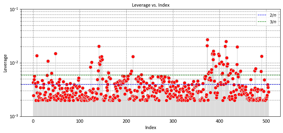
Let’s break down the interpretation based on some key observations:
Low Leverage Values (Close to 0):
Observations with low leverage values indicate that their predictor variable values are similar to the mean values of the predictor variables in the dataset.
These observations are not exerting a strong influence on the model’s predictions.
Moderate Leverage Values:
Observations with moderate leverage values have some deviation from the mean predictor variable values.
These observations contribute somewhat to the model’s predictions, but their influence is not extreme.
High Leverage Values (Close to 1):
Observations with high leverage values indicate that their predictor variable values are significantly different from the mean.
These observations have a strong impact on the model’s predictions, and their values could be driving the fitted line of the regression model.
Identifying High-Leverage Points:
\(2p/n\) as a Threshold:
Some statisticians use \(2p/n\) as a guideline to identify observations with high leverage. If the leverage value (\(h_{ii}\)) of an observation exceeds \(2p/n\), it is considered as potentially influential.
This guideline suggests that observations with leverage values that are at least twice the average leverage are worth examining closely, as they might have a strong impact on the model’s fit.
\(3p/n\) as a Threshold:
Some other statisticians use an even stricter threshold of \(3p/n\). If the leverage value (\(h_{ii}\)) of an observation exceeds \(3p/n\), it is flagged as potentially influential.
This threshold implies that an observation’s leverage needs to be significantly higher than the average to be considered influential.
Choosing between these thresholds can depend on the specific context of your analysis, the characteristics of your data, and the goals of your regression modeling. It’s important to note that these guidelines are not strict rules but rather heuristics to help identify observations that might be influential. Further investigation is usually necessary to determine whether these observations are indeed influential or if they should be treated as outliers.
import numpy as np

def calculate_cooks_distance(X, y):
    """
    Calculate Cook's distance for each observation.

    Parameters:
    X (numpy.ndarray): Input feature matrix with shape (n, p).
    y (numpy.ndarray): Target vector with shape (n,).

    Returns:
    numpy.ndarray: Array containing Cook's distance values for each observation.
    """

    # Calculate the coefficients using the normal equation
    coeff_matrix = np.linalg.inv(X.T @ X) @ (X.T @ y)

    # Calculate the predicted values
    y_pred = X @ coeff_matrix

    # Calculate the residuals
    residuals = y - y_pred

    # Calculate leverage values using the Moore-Penrose pseudo-inverse
    XTX_inverse = np.linalg.inv(X.T @ X)
    leverage_values = np.diagonal(X @ XTX_inverse @ X.T)

    # Get the shape of the input data
    n, p = X.shape

    # Calculate Mean Squared Error (MSE)
    MSE = np.mean(residuals**2)

    # Cook's distance calculation
    D = (residuals**2)/(p * MSE) * (leverage_values / ((1 - leverage_values)**2))

    return D

# Calculate Cook's distance
cook_distance = calculate_cooks_distance(X_with_intercept, y)

fig, ax = plt.subplots(1, 1, figsize=(9.5, 4.5))
n = X_with_intercept.shape[0]

markerline, stemlines, baseline = ax.stem(np.arange(n), cook_distance,
                                          linefmt='lightgrey', markerfmt='o')
_ = markerline.set_markerfacecolor('OrangeRed')
_ = ax.set(aspect = 'auto', xlabel = 'Index', ylabel = """Cook's Distance""",
           title = """Cook's Distance vs. Index""",
           yscale = 'log',  ylim = [1e-10, 1])
_ = ax.tick_params(axis='x', which='both', bottom=False, top=False)  # Remove x-axis ticks
_ = ax.axhline(y=np.mean(4/n), color='blue', linestyle='--', label= r'$4/n$')
_ = ax.legend()
# Fig setting
plt.tight_layout()
9.2.3.5. Modeling through statsmodels api#
Now, let’s summerize everything and do the above through statsmodels API [Seabold and Perktold, 2010]:
import statsmodels.api as sm

# Create the model matrix manually
X = Boston['LSTAT']  # Predictor variable (lstat)
# Response variable (medv)
y = Boston['MEDV']

X = sm.add_constant(X)  # Add an intercept term
display(X)

# Fit the simple linear regression model
Results = sm.OLS(y, X).fit()

# Print the model summary
print(Results.summary())
| const | LSTAT | |
|---|---|---|
| 0 | 1.0 | 4.98 |
| 1 | 1.0 | 9.14 |
| 2 | 1.0 | 4.03 |
| 3 | 1.0 | 2.94 |
| 4 | 1.0 | 5.33 |
| ... | ... | ... |
| 501 | 1.0 | 9.67 |
| 502 | 1.0 | 9.08 |
| 503 | 1.0 | 5.64 |
| 504 | 1.0 | 6.48 |
| 505 | 1.0 | 7.88 |
506 rows × 2 columns
                            OLS Regression Results
==============================================================================
Dep. Variable:                   MEDV   R-squared:                       0.544
Model:                            OLS   Adj. R-squared:                  0.543
Method:                 Least Squares   F-statistic:                     601.6
Date:                Wed, 08 Nov 2023   Prob (F-statistic):           5.08e-88
Time:                        14:31:08   Log-Likelihood:                -1641.5
No. Observations:                 506   AIC:                             3287.
Df Residuals:                     504   BIC:                             3295.
Df Model:                           1
Covariance Type:            nonrobust
==============================================================================
                 coef    std err          t      P>|t|      [0.025      0.975]
------------------------------------------------------------------------------
const         34.5538      0.563     61.415      0.000      33.448      35.659
LSTAT         -0.9500      0.039    -24.528      0.000      -1.026      -0.874
==============================================================================
Omnibus:                      137.043   Durbin-Watson:                   0.892
Prob(Omnibus):                  0.000   Jarque-Bera (JB):              291.373
Skew:                           1.453   Prob(JB):                     5.36e-64
Kurtosis:                       5.319   Cond. No.                         29.7
==============================================================================

Notes:
[1] Standard Errors assume that the covariance matrix of the errors is correctly specified.
The output is from the summary of a fitted linear regression model, which provides valuable information about the model’s coefficients, their standard errors, t-values, p-values, and confidence intervals. Let’s break down each component:
constandLSTAT: These are the variable names in the model.constrepresents the intercept (constant term), andLSTATrepresents the predictor variable.coef: This column displays the estimated coefficients of the linear regression model. Forconst, the estimated coefficient is 34.5538, and forLSTAT, it is -0.9500.std err: This column represents the standard errors of the coefficient estimates. It quantifies the uncertainty in the estimated coefficients. Forconst, the standard error is 0.563, and forLSTAT, it is 0.039.t: The t-values are obtained by dividing the coefficient estimates by their standard errors. The t-value measures how many standard errors the coefficient estimate is away from zero. Forconst, the t-value is 61.415, and forLSTAT, it is -24.528.P>|t|: This column provides the p-values associated with the t-values. The p-value represents the probability of observing a t-value as extreme as the one calculated, assuming the null hypothesis that the coefficient is equal to zero. Lower p-values indicate stronger evidence against the null hypothesis. In this case, both coefficients have extremely low p-values (close to 0), indicating that they are statistically significant.[0.025 0.975]: These are the lower and upper bounds of the 95% confidence intervals for the coefficients. The confidence intervals provide a range of plausible values for the true population coefficients. Forconst, the confidence interval is [33.448, 35.659], and forLSTAT, it is [-1.026, -0.874].
The coefficient estimates indicate how the response variable (medv) is expected to change for a one-unit increase in the predictor variable (lstat). The low p-values and confidence intervals not containing zero suggest that both the intercept and LSTAT coefficient are statistically significant and have a significant impact on the response variable.
# OLS Reression results
def Reg_Result(Inp):
    Temp = pd.read_html(Inp.summary().tables[1].as_html(), header=0, index_col=0)[0]
    display(Temp.style\
    .format({'coef': '{:.4e}', 'P>|t|': '{:.4e}', 'std err': '{:.4e}'})\
    .bar(subset=['coef'], align='mid', color='Lime')\
    .set_properties(subset=['std err'], **{'background-color': 'DimGray', 'color': 'White'}))

Reg_Result(Results)
| coef | std err | t | P>|t| | [0.025 | 0.975] | |
|---|---|---|---|---|---|---|
| const | 3.4554e+01 | 5.6300e-01 | 61.415000 | 0.0000e+00 | 33.448000 | 35.659000 |
| LSTAT | -9.5000e-01 | 3.9000e-02 | -24.528000 | 0.0000e+00 | -1.026000 | -0.874000 |
def _regplot(ax, results, *args, **kwargs):
    '''
    y  = beta_1 *x + beta_0
    '''
    b0 = results.params['const']
    b1 = results.params['LSTAT']
    xlim = ax.get_xlim()
    ylim = [b1 * xlim[0] + b0, b1 * xlim[1] + b0]
    ax.plot(xlim, ylim, *args, **kwargs)

fig, ax = plt.subplots(3, 2, figsize=(9.5, 12), sharex  = False, sharey = False)
ax = ax.ravel()

# regplot
_ = ax[0].scatter(x= Boston.LSTAT, y= Boston.MEDV, fc= 'SkyBlue', ec = 'k', s = 50,
                    label='Original Data')
_ = ax[0].set(xlabel = 'LSTAT', ylabel = 'MEDV',
              xlim = [-10, 50], ylim = [0, 60], title = 'Linear Regression')
_regplot(ax = ax[0], results = Results,
         linestyle = 'dashed', color = 'red', lw = 3, label='Fitted Line')
_ = ax[0].legend()
# residuals
_ = ax[1].scatter(Results.fittedvalues, Results.resid, fc='none', ec = 'DarkRed', s = 50)
_ = ax[1].axhline(0, c='k', ls='--')
_ = ax[1].set(aspect = 'auto',
              xlabel = 'Fitted value',
              ylabel = 'Residual',
              xlim = [0, 40], ylim = [-20, 30], title = 'Residuals for Linear Regression')
# leverage (Optional Content)
gs = ax[2].get_gridspec()
for i in range(2,4):
    ax[i].remove()
ax3 = fig.add_subplot(gs[1, :])
infl = Results.get_influence()
markerline, stemlines, baseline = ax3.stem(np.arange(X.shape[0]), infl.hat_matrix_diag,
                                             linefmt='lightgrey', markerfmt='o')
_ = markerline.set_markerfacecolor('red')
_ = ax3.set(aspect = 'auto', xlabel = 'Index', ylabel = 'Leverage',
            title = 'Leverage vs. Index',
            yscale = 'log',  ylim = [1e-3, 1e-1])
_ = ax3.tick_params(axis='x', which='both', bottom=False, top=False)  # Remove x-axis ticks
_ = ax3.axhline(y=np.mean(2/n), color='blue', linestyle='--', label= r'$2/n$')
_ = ax3.axhline(y=np.mean(3/n), color='green', linestyle='--', label= r'$3/n$')
_ = ax3.legend()

# Cook's Distance (Optional Content)
gs = ax[4].get_gridspec()
for i in range(4,6):
    ax[i].remove()
ax4 = fig.add_subplot(gs[2, :])
markerline, stemlines, baseline = ax4.stem(np.arange(X.shape[0]), infl.cooks_distance[0],
                                             linefmt='lightgrey', markerfmt='o')
_ = markerline.set_markerfacecolor('OrangeRed')
_ = ax4.set(aspect = 'auto', xlabel = 'Index', ylabel = """Cook's Distance""",
            title = """Cook's Distance vs. Index""",
            yscale = 'log',  ylim = [1e-10, 1])
_ = ax4.tick_params(axis='x', which='both', bottom=False, top=False)  # Remove x-axis ticks
_ = ax4.axhline(y=np.mean(2/n), color='blue', linestyle='--', label= r'$2/n$')
_ = ax4.axhline(y=np.mean(3/n), color='green', linestyle='--', label= r'$3/n$')
_ = ax4.legend()
# Fig setting

# Fig setting
plt.tight_layout()
9.2.4. Linear Regression through sklearn API#
One can also execute a straightforward linear regression analysis by employing the LinearRegression model available in the sklearn library [scikit-learn Developers, 2023]. The following delineates the procedure:
from sklearn.linear_model import LinearRegression
# Prepare the predictor and response variables
X = Boston[['LSTAT']]  # Predictor variable (lstat)
y = Boston['MEDV']  # Response variable (medv)

# Create and fit the Linear Regression model
reg = LinearRegression()
_ = reg.fit(X, y)

# Print the model coefficients and intercept
print(f"Intercept (const): {reg.intercept_}")
print(f"Coefficient (LSTAT): {reg.coef_[0]}")
Intercept (const): 34.55384087938311
Coefficient (LSTAT): -0.9500493537579909
In this code, we use sklearn to perform the simple linear regression. We first read the dataset as before, then prepare the predictor variable X (lstat) and the response variable y (medv). We create an instance of the LinearRegression model and fit it to the data using model.fit(X, y).
After fitting the model, we can access the model’s coefficients using model.coef_, which gives us the coefficient for the predictor variable LSTAT, and model.intercept_, which gives us the intercept (constant term). The coefficients obtained here should match the ones we got from the statsmodels library earlier.
Example: The dataset used in this example comprises monthly mean temperature data for ‘CALGARY INT’L A’. Our objective is to identify linear trendlines for each of the 12 months, spanning the period from 1881 to 2012.
import pandas as pd
Link = 'https://climate.weather.gc.ca/climate_data/bulk_data_e.html?format=csv&stationID=2205&Year=2000&Month=1&Day=1&time=&timeframe=3&submit=Download+Data'

df = pd.read_csv(Link, usecols = ['Date/Time', 'Year', 'Month' , 'Mean Temp (°C)'])
df['Date/Time'] = pd.to_datetime(df['Date/Time'])
df = df.rename(columns = {'Date/Time':'Date'})
display(df)
| Date | Year | Month | Mean Temp (°C) | |
|---|---|---|---|---|
| 0 | 1881-01-01 | 1881 | 1 | NaN |
| 1 | 1881-02-01 | 1881 | 2 | NaN |
| 2 | 1881-03-01 | 1881 | 3 | NaN |
| 3 | 1881-04-01 | 1881 | 4 | NaN |
| 4 | 1881-05-01 | 1881 | 5 | NaN |
| ... | ... | ... | ... | ... |
| 1574 | 2012-03-01 | 2012 | 3 | 0.7 |
| 1575 | 2012-04-01 | 2012 | 4 | 5.2 |
| 1576 | 2012-05-01 | 2012 | 5 | 9.6 |
| 1577 | 2012-06-01 | 2012 | 6 | 13.7 |
| 1578 | 2012-07-01 | 2012 | 7 | 18.3 |
1579 rows × 4 columns
import matplotlib.pyplot as plt
from sklearn.linear_model import LinearRegression
import calendar

def _regplot(ax, df_sub, X, reg, *args, **kwargs):
    '''
    Plots the regression line on the given axis.

    Parameters:
    - ax: matplotlib axis
        The axis to plot on.
    - df_sub: pandas DataFrame
        Subset of data for a specific month.
    - X: numpy array
        Independent variable (index values).
    - reg: regression model
        The regression model used for prediction.
    - *args, **kwargs: additional plot arguments
        Additional arguments for the plot function.
    '''
    y_hat = reg.predict(X)
    ax.plot(df_sub.Date, y_hat, *args, **kwargs)
    ax.set_title(f'Slope = {reg.coef_.ravel()[0]:.3}', fontsize=14)

fig, axes = plt.subplots(12, 1, figsize=(9.5, 20), sharex=True)
for m, ax in enumerate(axes, start=1):
    # Create and fit the Linear Regression model
    reg = LinearRegression()
    # Subset data for a specific month
    df_sub = df.loc[df.Month == m].reset_index(drop=True)

    # Scatter plot for Mean Max Temp
    ax.scatter(df_sub['Date'], df_sub['Mean Temp (°C)'],
               fc='Blue', ec='k', s=15, label = 'Mean Temp (°C)')

    # Set axis label as the month name
    ax.set_ylabel(calendar.month_name[m], weight='bold')
    ax.grid(True)

    # Remove rows with missing values
    df_sub = df_sub.dropna()

    # Prepare data for linear regression
    X = df_sub.index.values.reshape(-1, 1)
    y = df_sub['Mean Temp (°C)'].values.reshape(-1, 1)

    # Create and fit a Linear Regression model
    reg = LinearRegression()
    _ = reg.fit(X, y)

    # Plot the fitted line
    _regplot(ax=ax, df_sub=df_sub, X=X, reg=reg,
             linestyle='dashed', color='red', lw=1.5, label='Fitted Line')
    ax.legend()

    # Set four y-ticks
    yticks = np.linspace(df_sub['Mean Temp (°C)'].min()-3, df_sub['Mean Temp (°C)'].max()+3, 4)
    yticks = np.round(yticks, 1)
    ax.set_yticks(yticks)

fig.suptitle("""Monthly Mean Temperature (°C) Trends at CALGARY INT'L A: Linear Analysis""", y = 0.99,
            weight = 'bold', fontsize = 16)
plt.tight_layout()
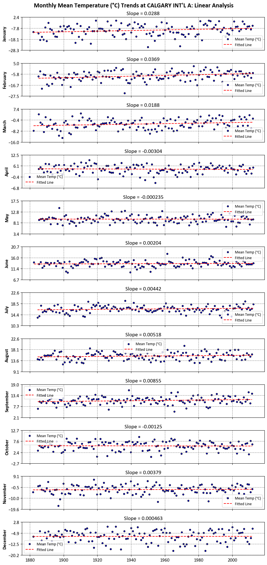
Note
Please note that all the slopes shown in the figure above have been provided with three significant decimal places.
9.2.5. Analyzing Long-Term Trends#
When analyzing trends in data, it’s important to consider the significance of the observed trendlines, and p-values play a crucial role in this context. A p-value is a statistical measure that helps determine the significance of a trend or relationship observed in a dataset. In the context of the provided trendlines for mean monthly temperatures at Calgary International Airport, it would be advisable to conduct a statistical test to evaluate the significance of these trends.
To assess the significance of these trendlines and whether they are statistically meaningful, you would typically perform a linear regression analysis and calculate p-values for each trendline. Here’s a brief note on the significance of these trendlines and p-values:
Note on P-Values and Significance of Trendlines:
In the analysis of the mean monthly temperature trends at Calgary International Airport, we have calculated the slopes of linear trendlines to understand how temperatures are changing over time. However, to determine whether these observed trends are statistically significant, we need to consider p-values.
P-Values: A p-value measures the probability of obtaining the observed trendlines (or more extreme ones) if there were no actual trends in the data. Lower p-values indicate stronger evidence against the null hypothesis, suggesting that the observed trend is not due to random chance.
Significance: To assess the significance of these trendlines, we typically perform linear regression analysis. In this analysis, each month’s temperature data is regressed against time (the independent variable). The p-value associated with each trendline quantifies the likelihood of observing the reported trend under the assumption that there is no true linear relationship between time and temperature.
Interpretation: A low p-value (typically, below a significance level like 0.05) suggests that the trend is statistically significant. In other words, it provides evidence that the temperature changes observed for that month are not just random fluctuations.
Caution: It’s important to be cautious when interpreting p-values. While a low p-value indicates statistical significance, it does not by itself establish the practical or real-world significance of the trend. Additionally, trends can be affected by many factors, and further analysis is needed to understand the underlying causes of temperature changes.
Several Python packages can calculate p-values for linear regression. Here are some commonly used ones:
StatsModels
SciPy
PyStatsModels
etc.
Example:
import matplotlib.pyplot as plt
from scipy import stats
import calendar

slope_list = []
month_list = []
p_val_list = []

for m in range(1, 13):
    df_sub = df.loc[df.Month == m].reset_index(drop=True).dropna()
    X = df_sub.index.values
    y = df_sub['Mean Temp (°C)'].values
    slope, _, _, p_value, _ = stats.linregress(X, y)
    slope_list.append(slope)
    month_list.append(calendar.month_name[m])
    p_val_list.append(p_value)
    del df_sub, X, y, slope, p_value

df_results = pd.DataFrame({'Slope':slope_list, 'p-value':p_val_list}, index = month_list)
The following table represents the slopes of linear trendlines for the mean monthly temperature at Calgary International Airport weather stations from January 1881 to July 2012. Additionally, p-values are provided to assess the significance of these trends.
display(df_results)
| Slope | p-value | |
|---|---|---|
| January | 0.028849 | 0.019986 |
| February | 0.036869 | 0.000755 |
| March | 0.018809 | 0.025253 |
| April | -0.003040 | 0.601981 |
| May | -0.000235 | 0.948623 |
| June | 0.002036 | 0.517881 |
| July | 0.004418 | 0.142400 |
| August | 0.005177 | 0.151559 |
| September | 0.008547 | 0.067413 |
| October | -0.001246 | 0.796791 |
| November | 0.003791 | 0.684526 |
| December | 0.000463 | 0.962145 |
Each slope corresponds to a specific month and represents the rate of change in temperature over time, expressed in degrees Celsius per year. Let’s break down the information, explain the slope, and discuss the significance at different confidence levels.
January (0.028849): The positive slope indicates an increasing trend in mean temperatures in January over the years. At a 90% confidence level, this trend is significant, as the p-value (0.019986) is less than 0.1.
February (0.036869): This positive slope suggests a significant increase in mean temperatures in February. The very low p-value (0.000755) indicates significance even at a 99% confidence level.
March (0.018809): The positive slope implies a gradual rise in March temperatures. At a 90% confidence level, this trend is significant (p-value: 0.025253).
April (-0.003040): The negative slope suggests a slight decrease in mean temperatures in April, although it is not statistically significant at any of the specified confidence levels. The p-value is relatively high (0.601981).
May (-0.000235): Similarly, the small negative slope in May temperatures is not statistically significant at any confidence level (p-value: 0.948623).
June (0.002036): The positive slope indicates a minor increase in June temperatures, but it’s not statistically significant at any confidence level (p-value: 0.517881).
July (0.004418): This positive slope suggests a small but significant increase in July temperatures at a 90% confidence level, as the p-value is 0.142400.
August (0.005177): Like July, August also shows a slight but statistically significant increase in temperatures at a 90% confidence level (p-value: 0.151559).
September (0.008547): The positive slope for September indicates a more significant increase in temperatures. This trend is significant at a 90% confidence level (p-value: 0.067413).
October (-0.001246): The small negative slope in October temperatures is not statistically significant at any of the confidence levels (p-value: 0.796791).
November (0.003791): This positive slope suggests a slight increase in November temperatures, but it is not statistically significant at any confidence level (p-value: 0.684526).
December (0.000463): The positive slope for December indicates a very slight increase in temperatures, but it’s not statistically significant at any confidence level (p-value: 0.962145).
These slopes provide insights into the long-term temperature trends for each month at the Calgary International Airport weather stations. Positive slopes indicate warming trends, negative slopes indicate cooling trends, and the magnitude of the slope reflects the rate of change.