10.4. Regression Trees and Linear Models (Optional Section)#
When we compare regression and classification trees to traditional methods, the differences become quite pronounced, especially when we contrast them with linear models, particularly linear regression [James et al., 2023].
10.4.1. Linear Regression#
Linear regression is a statistical modeling technique grounded in a linear relationship between the predictor variables (\(X_1, X_2, \ldots, X_p\)) and the predicted outcome (\(f(X)\)). The model is expressed by the equation:
Here, \(\beta_0\) is the intercept term, and \(\beta_j\) are the coefficients associated with each predictor variable. The predicted outcome \(f(X)\) is a linear combination of these variables and their respective coefficients. This linear approach is particularly effective when the underlying relationships in the data can be accurately represented by a straight line.
10.4.2. Regression Trees#
In contrast, regression trees adopt a distinctive modeling structure. The predictive function \(f(X)\) for regression trees is defined as follows:
In this equation, \(M\) represents the number of terminal nodes or regions in the tree, \(c_m\) denotes the constant associated with the \(m\)-th region, and \(\mathbb{I}_{X\in R_m}\) is an indicator function that equals 1 if \(X\) falls within region \(R_m\) and 0 otherwise. Unlike linear regression, regression trees accommodate non-linear relationships in the data by partitioning the feature space into distinct regions, each associated with a unique constant.
10.4.3. Key Distinctions#
The fundamental distinction lies in the modeling approach. Linear regression assumes a linear relationship between the predictors and the response, making it suitable for linearly structured data. On the other hand, regression trees offer flexibility in capturing non-linear patterns by segmenting the feature space. The choice between these methods depends on the nature of the data and the underlying relationships one aims to capture. While linear regression is straightforward and interpretable, regression trees excel in capturing complex, non-linear dependencies within the data.
Note
The indicator function, denoted as \( \mathbb{I}_A \) or \( 1_A \), is defined for a set \( A \) and takes values in the real numbers. Its primary function is to serve as a binary indicator, representing the membership or non-membership of an element in the set \( A \).
Mathematically, the indicator function is expressed as follows:
In this formulation, the function evaluates to 1 when the input \( x \) is an element of the set \( A \), and it evaluates to 0 otherwise. This binary nature makes the indicator function a valuable tool in defining and manipulating sets within various mathematical contexts.
10.4.4. Example: Material Strength Prediction#
Example: Suppose we have a fictional dataset that relates the temperature (\(X\)) to the strength of a material (\(y\)). We want to predict the material strength under different temperatures using linear regression and decision tree regression.
import numpy as np
import matplotlib.pyplot as plt
from sklearn.linear_model import LinearRegression
import seaborn as sns

# Set the style for a more visually appealing plot
plt.style.use('../mystyle.mplstyle')

# Generate synthetic data
np.random.seed(42)
temperature = 50 * np.random.rand(100, 1)
strength = 20 + 0.5 * temperature + np.random.randn(100, 1) * 5

# Create a scatter plot with enhanced style
fig, ax = plt.subplots(figsize=(9.5, 5.5))

# Scatter plot with color-coded points based on material strength
_ = ax.scatter(temperature, strength, c=strength.flatten(),
                     cmap='Blues', edgecolor='k', linewidth=1, s=80, alpha=0.8)

# Set axis labels and plot title
ax.set(xlabel='Temperature (°C)', ylabel='Material Strength')

# Set a bold title with a larger font size
ax.set_title('Material Strength vs. Temperature', fontsize=14, weight='bold')

# Ensure a tight layout for better presentation
plt.tight_layout()
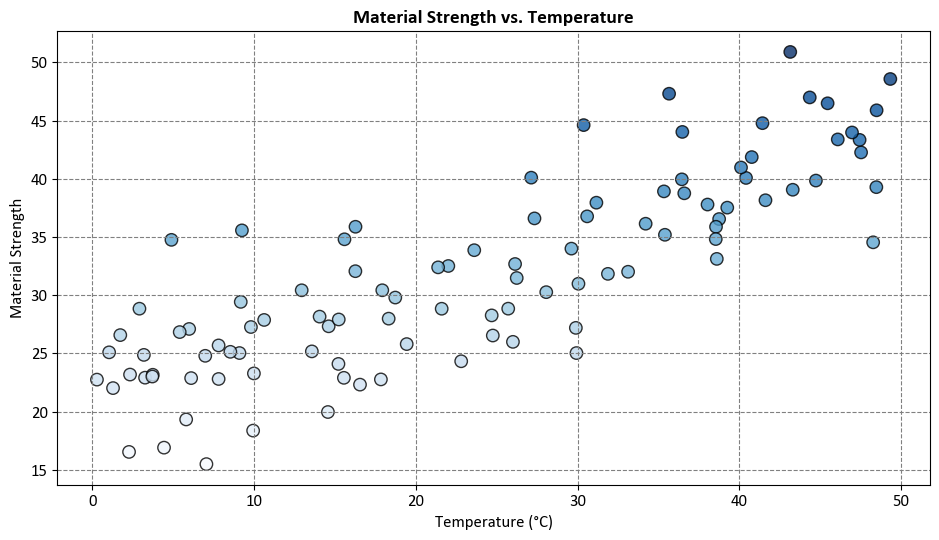
In this example, we simulate a scenario where material strength has a linear relationship with temperature, but there is some variability due to other factors, represented by the random noise.
import numpy as np
import matplotlib.pyplot as plt
from sklearn.linear_model import LinearRegression
from sklearn.tree import DecisionTreeRegressor
import seaborn as sns

# Set the style for a more visually appealing plot
plt.style.use('../mystyle.mplstyle')

# Generate synthetic data
np.random.seed(42)
temperature = 50 * np.random.rand(100, 1)
strength = 20 + 0.5 * temperature + np.random.randn(100, 1) * 5

# Create a scatter plot with enhanced style
fig, ax = plt.subplots(figsize=(9.5, 5.5))

# Scatter plot with color-coded points based on material strength
_ = ax.scatter(temperature, strength, c=strength.flatten(),
               cmap='Blues', edgecolor='k', linewidth=1, s=80, alpha=0.8, label='Actual Data')

# Fit and plot the linear regression line
lin_reg = LinearRegression().fit(temperature, strength)
_ = ax.plot(temperature, lin_reg.predict(temperature),
            linestyle='-', color='OrangeRed',
            label='Linear Regression Line', linewidth=2)

# Train a decision tree regression model
tree_reg = DecisionTreeRegressor(max_depth=3)
tree_reg.fit(temperature, strength)

# Plot the decision tree regression prediction
temperature_test = np.arange(0.0, 50.0, 1)[:, np.newaxis]
strength_pred = tree_reg.predict(temperature_test)

_ = ax.plot(temperature_test, strength_pred,
            linestyle='-', color='Purple',
            label='Decision Tree Prediction', linewidth=2)

# Set axis labels and plot title
ax.set(xlabel='Temperature (°C)', ylabel='Material Strength')

# Add legend
ax.legend(fontsize=12)

# Set a bold title with a larger font size
ax.set_title('Material Strength Prediction Comparison', fontsize=14, weight='bold')

# Ensure a tight layout for better presentation
plt.tight_layout()
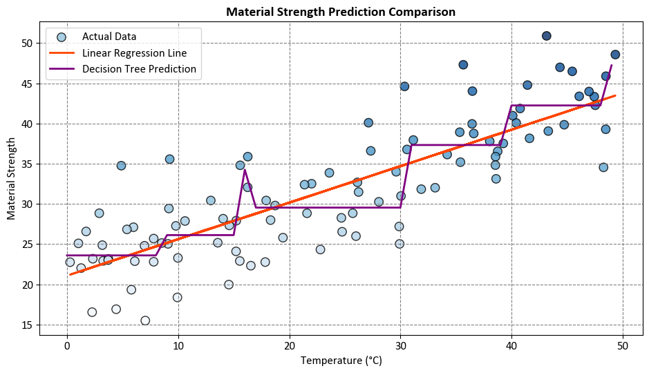
Comparison:
Linear regression assumes a linear relationship and provides a straightforward interpretation. In our example, the linear regression line captures the overall trend of increasing material strength with temperature.
On the other hand, the decision tree regression accommodates non-linear patterns. In this example, it may capture abrupt changes in material strength at specific temperature thresholds.
The choice between linear regression and decision tree regression depends on the underlying characteristics of the data and the complexity of the relationship between variables. Linear regression is suitable for capturing linear trends, while decision tree regression can handle non-linear relationships and capture more intricate patterns in the data.
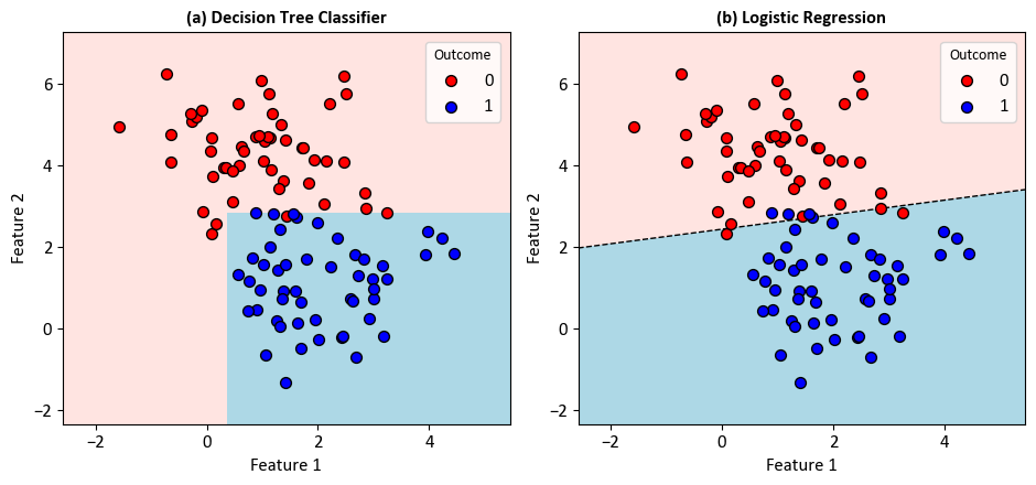
10.4.5. Example - Binary Classification#
Example - Binary Classification: Consider a scenario wherein a dataset comprises data points inherently categorized into two distinct classes.
import numpy as np
from sklearn.datasets import make_blobs
from sklearn.linear_model import LogisticRegression
from sklearn.tree import DecisionTreeClassifier
from matplotlib.colors import ListedColormap
from sklearn.inspection import DecisionBoundaryDisplay
from sklearn import tree
import matplotlib.pyplot as plt
# Display the equation using LaTeX
from IPython.display import Latex, display

def print_bold(txt, c = 31):
    print(f"\033[1;{c}m" + txt + "\033[0m")

# Use a custom style for plotting
plt.style.use('../mystyle.mplstyle')

# Define colors and colormap for the plot
colors = ["Red", "Blue"]
cmap_light = ListedColormap(["MistyRose", "LightBlue"])

# Generate synthetic data using make_blobs
n_samples = 100
n_features = 2
centers = 2
cluster_std = 1.0
X, y = make_blobs(n_samples=n_samples, n_features=n_features, centers=centers, random_state=0, cluster_std=cluster_std)

# Create subplots for decision boundary visualization
fig, axes = plt.subplots(1, 2, figsize=(9.5, 4.5))
axes = axes.ravel()

# Define parameters for classifiers
dts_parms = {'max_depth': 2, 'max_features': None, 'max_leaf_nodes': None}
lr_parms = {'max_iter': 50, 'solver': 'lbfgs'}

# Create classifier instances
models = [DecisionTreeClassifier(**dts_parms), LogisticRegression(**lr_parms)]
model_names = ['Decision Tree Classifier', 'Logistic Regression']
model_alphs = 'ab'

# Iterate through classifiers and plot decision boundaries
for ax, classifier, name, code in zip(axes, models, model_names, model_alphs):
    # Fit the classifier to the data
    classifier.fit(X, y)

    # Plot decision boundary using DecisionBoundaryDisplay
    DecisionBoundaryDisplay.from_estimator(classifier, X, cmap=cmap_light, ax=ax,
                                           response_method="predict",
                                           grid_resolution= 500,
                                           plot_method="pcolormesh",
                                           xlabel='Feature 1', ylabel='Feature 2',
                                           shading="auto")

    # Scatter plot for data points
    for num in np.unique(y):
        ax.scatter(X[:, 0][y == num], X[:, 1][y == num], c=colors[num],
                   s=50, edgecolors='k', label=str(num), zorder = 2)

    # Set legend and title for the subplot
    ax.legend(title='Outcome', fontsize=12)
    ax.set_title(f'({code}) {name}', weight='bold')
    ax.grid(False)

    # For DecisionTreeClassifier
    if isinstance(classifier, DecisionTreeClassifier):
        print_bold('Decision Tree Classifier:')
        print(tree.export_text(classifier,
                               feature_names = [f'Feature_{i + 1}' for i in range(2)]))

    # For Logistic Regression, get the coefficients and intercept
    if isinstance(classifier, LogisticRegression):
        print_bold('Logistic Regression:')
        coef = classifier.coef_[0]
        intercept = classifier.intercept_
        # Plot the decision boundary as a dashed line
        x_vals = np.linspace(ax.get_xlim()[0], ax.get_xlim()[1], 100)
        y_vals = (-coef[0] / coef[1]) * x_vals - (intercept[0] / coef[1])
        ax.plot(x_vals, y_vals, '--k', label='Decision Boundary (Logistic Regression)', zorder = 1)
        equation = f'$Feature_2 = {(-coef[0] / coef[1]):+.3f} * Feature_1 {(intercept[0] / coef[1]):+.3f}$'
        display(Latex(equation))

# Adjust layout for better visualization
plt.tight_layout()
Decision Tree Classifier:
|--- Feature_2 <= 2.85
|   |--- Feature_1 <= 0.36
|   |   |--- class: 0
|   |--- Feature_1 >  0.36
|   |   |--- class: 1
|--- Feature_2 >  2.85
|   |--- class: 0

Logistic Regression:
Note
The decision boundary line in logistic regression is derived from the logistic function. In logistic regression with two variables (features), the decision boundary can be expressed as a linear combination of the features. The logistic function is used to transform this linear combination into a probability.
The logistic regression hypothesis function is given by:
Here:
\(P(X)\) is the predicted probability that the example \(x\) belongs to the positive class.
\(\beta_0, \beta_1, \beta_2\) are the parameters (intercept and coefficients).
\(X = (x_1, x_2)\) are the input features.
To find the decision boundary, we set \(h_{\beta}(x)\) to 0.5 (as this is the threshold for classification in binary logistic regression). The logistic function maps any real-valued number to the range [0, 1]. Therefore:
Solving this equation for \(x_2\) gives the equation of the decision boundary:
This is the equation of a straight line in a two-dimensional space. If you solve for \(x_2\), you get:
This is the equation of the decision boundary line. In the provided code, \(x_1\) is represented by x_vals, and \(x_2\) is represented by y_vals. The coefficients and intercept from the logistic regression model are used to calculate these values for plotting the decision boundary.
10.4.5.1. Comparison#
import numpy as np
import pandas as pd
from sklearn.model_selection import StratifiedKFold
from sklearn import metrics
from sklearn.tree import DecisionTreeClassifier
from sklearn.linear_model import LogisticRegression

# Function to print a line of underscores for separation
def _Line(n = 60, c = '_'):
    print(n * c)

def print_bold(txt, c = 31):
    print(f"\033[1;{c}m" + txt + "\033[0m")

# Sample data X and y are assumed to be defined here

# Models to be evaluated
model_alphs = 'ab'

# Loop through each model
for model, name, alph in zip(models, model_names, model_alphs):
    _Line(n = 80, c = '=')
    print_bold(f'({alph}) {name}', c = 34)
    _Line(n = 80, c = '=')

    # Initialize KFold cross-validator
    n_splits = 5
    skf = StratifiedKFold(n_splits=n_splits, shuffle=True, random_state=42)
    # The splitt would be 80-20!

    # Lists to store train and test scores for each fold
    train_acc_scores, test_acc_scores, train_f1_scores, test_f1_scores = [], [], [], []
    train_class_proportions, test_class_proportions = [], []

    # DataFrames to store classification reports
    reports_train = pd.DataFrame()
    reports_test = pd.DataFrame()

    # Perform Cross-Validation
    for fold, (train_idx, test_idx) in enumerate(skf.split(X, y), 1):
        X_train, X_test = X[train_idx], X[test_idx]
        y_train, y_test = y[train_idx], y[test_idx]
        model.fit(X_train, y_train)

        # Calculate class proportions for train and test sets
        train_class_proportions.append([np.mean(y_train == model) for model in np.unique(y)])
        test_class_proportions.append([np.mean(y_test == model) for model in np.unique(y)])

        # train
        y_train_pred = model.predict(X_train)
        train_acc_scores.append(metrics.accuracy_score(y_train, y_train_pred))
        train_f1_scores.append(metrics.f1_score(y_train, y_train_pred, average = 'weighted'))

        # test
        y_test_pred = model.predict(X_test)
        test_acc_scores.append(metrics.accuracy_score(y_test, y_test_pred))
        test_f1_scores.append(metrics.f1_score(y_test, y_test_pred, average = 'weighted'))

    _Line()
    #  Print the Train and Test Scores for each fold
    for fold in range(n_splits):
        print_bold(f'Fold {fold + 1}:')
        print(f"\tTrain Class Proportions: {train_class_proportions[fold]}*{len(y_train)}")
        print(f"\tTest Class Proportions: {test_class_proportions[fold]}*{len(y_test)}")
        print(f"\tTrain Accuracy Score = {train_acc_scores[fold]:.4f}, Test Accuracy Score = {test_acc_scores[fold]:.4f}")
        print(f"\tTrain F1 Score (weighted) = {train_f1_scores[fold]:.4f}, Test F1 Score (weighted)= {test_f1_scores[fold]:.4f}")

    _Line()
    print_bold('Accuracy Score:')
    print(f"\tMean Train Accuracy Score: {np.mean(train_acc_scores):.4f} ± {np.std(train_acc_scores):.4f}")
    print(f"\tMean Test Accuracy Score: {np.mean(test_acc_scores):.4f} ± {np.std(test_acc_scores):.4f}")
    print_bold('F1 Score:')
    print(f"\tMean F1 Accuracy Score (weighted): {np.mean(train_f1_scores):.4f} ± {np.std(train_f1_scores):.4f}")
    print(f"\tMean F1 Accuracy Score (weighted): {np.mean(test_f1_scores):.4f} ± {np.std(test_f1_scores):.4f}")
    _Line()
================================================================================
(a) Decision Tree Classifier
================================================================================
____________________________________________________________
Fold 1:
	Train Class Proportions: [0.5, 0.5]*80
	Test Class Proportions: [0.5, 0.5]*20
	Train Accuracy Score = 1.0000, Test Accuracy Score = 0.9500
	Train F1 Score (weighted) = 1.0000, Test F1 Score (weighted)= 0.9499
Fold 2:
	Train Class Proportions: [0.5, 0.5]*80
	Test Class Proportions: [0.5, 0.5]*20
	Train Accuracy Score = 0.9875, Test Accuracy Score = 1.0000
	Train F1 Score (weighted) = 0.9875, Test F1 Score (weighted)= 1.0000
Fold 3:
	Train Class Proportions: [0.5, 0.5]*80
	Test Class Proportions: [0.5, 0.5]*20
	Train Accuracy Score = 0.9875, Test Accuracy Score = 0.9500
	Train F1 Score (weighted) = 0.9875, Test F1 Score (weighted)= 0.9499
Fold 4:
	Train Class Proportions: [0.5, 0.5]*80
	Test Class Proportions: [0.5, 0.5]*20
	Train Accuracy Score = 0.9875, Test Accuracy Score = 1.0000
	Train F1 Score (weighted) = 0.9875, Test F1 Score (weighted)= 1.0000
Fold 5:
	Train Class Proportions: [0.5, 0.5]*80
	Test Class Proportions: [0.5, 0.5]*20
	Train Accuracy Score = 0.9875, Test Accuracy Score = 0.9500
	Train F1 Score (weighted) = 0.9875, Test F1 Score (weighted)= 0.9499
____________________________________________________________
Accuracy Score:
	Mean Train Accuracy Score: 0.9900 ± 0.0050
	Mean Test Accuracy Score: 0.9700 ± 0.0245
F1 Score:
	Mean F1 Accuracy Score (weighted): 0.9900 ± 0.0050
	Mean F1 Accuracy Score (weighted): 0.9699 ± 0.0246
____________________________________________________________
================================================================================
(b) Logistic Regression
================================================================================
____________________________________________________________
Fold 1:
	Train Class Proportions: [0.5, 0.5]*80
	Test Class Proportions: [0.5, 0.5]*20
	Train Accuracy Score = 0.9375, Test Accuracy Score = 0.9500
	Train F1 Score (weighted) = 0.9375, Test F1 Score (weighted)= 0.9499
Fold 2:
	Train Class Proportions: [0.5, 0.5]*80
	Test Class Proportions: [0.5, 0.5]*20
	Train Accuracy Score = 0.9250, Test Accuracy Score = 1.0000
	Train F1 Score (weighted) = 0.9250, Test F1 Score (weighted)= 1.0000
Fold 3:
	Train Class Proportions: [0.5, 0.5]*80
	Test Class Proportions: [0.5, 0.5]*20
	Train Accuracy Score = 0.9250, Test Accuracy Score = 0.9500
	Train F1 Score (weighted) = 0.9250, Test F1 Score (weighted)= 0.9499
Fold 4:
	Train Class Proportions: [0.5, 0.5]*80
	Test Class Proportions: [0.5, 0.5]*20
	Train Accuracy Score = 0.9125, Test Accuracy Score = 0.9500
	Train F1 Score (weighted) = 0.9125, Test F1 Score (weighted)= 0.9499
Fold 5:
	Train Class Proportions: [0.5, 0.5]*80
	Test Class Proportions: [0.5, 0.5]*20
	Train Accuracy Score = 0.9625, Test Accuracy Score = 0.8500
	Train F1 Score (weighted) = 0.9625, Test F1 Score (weighted)= 0.8496
____________________________________________________________
Accuracy Score:
	Mean Train Accuracy Score: 0.9325 ± 0.0170
	Mean Test Accuracy Score: 0.9400 ± 0.0490
F1 Score:
	Mean F1 Accuracy Score (weighted): 0.9325 ± 0.0170
	Mean F1 Accuracy Score (weighted): 0.9398 ± 0.0491
____________________________________________________________
The outcomes present an evaluation of two models: a decision tree classifier and a logistic regression. Both models employ accuracy and F1 score as performance indicators. Accuracy reflects the proportion of correctly classified instances, while the F1 score serves as the harmonic mean of precision and recall, both metrics ranging from 0 to 1, with higher values denoting superior performance.
These results stem from a five-fold stratified cross-validation, ensuring random data division into five subsets, each maintaining class proportions akin to the original dataset. For each fold, one subset acts as the test set, with the remaining four constituting the training set. Model performance is then averaged across these five folds.
Key observations for result interpretation include:
The decision tree classifier outperforms the logistic regression, exhibiting higher mean accuracy and F1 score on both training and test sets. This suggests the decision tree classifier’s suitability for the given data.
The decision tree classifier demonstrates minimal standard deviations for both metrics, indicating consistent performance across diverse folds. Conversely, the logistic regression manifests higher standard deviations, particularly for the test set, signifying more variable performance across folds.
The decision tree classifier achieves a notably high mean accuracy and F1 score on the training set, approaching 1. This signifies adept fitting to the training data but raises concerns of potential overfitting. In contrast, the logistic regression, while less prone to overfitting, displays lower mean accuracy and F1 score on the training set, implying potential underfitting and a lesser grasp of data complexity.
As anticipated, the decision tree classifier exhibits a slightly lower mean accuracy and F1 score on the test set compared to the training set, indicative of overfitting. Conversely, the logistic regression displays a somewhat higher mean accuracy and F1 score on the test set, an uncommon occurrence that may be attributed to random variation or sampling error.
The findings suggest the decision tree classifier surpasses the logistic regression on this data, albeit with potential overfitting. The logistic regression, while less prone to overfitting, might face underfitting challenges. To enhance both models, exploring different hyperparameters, feature selection, or regularization techniques is advised. Additionally, considering alternative metrics, such as ROC curve or confusion matrix, could provide a more comprehensive model comparison.
Note
metrics.accuracy_scoreis a function commonly used in the context of classification tasks within the field of machine learning. It is part of the scikit-learn library in Python. This function is utilized to quantify the accuracy of a classification model by comparing the predicted labels against the true labels of a dataset.The accuracy score is calculated by dividing the number of correctly classified instances by the total number of instances. Mathematically, it can be expressed as:
(10.25)#\[\begin{equation} \text{Accuracy} = \frac{\text{Number of Correctly Classified Instances}}{\text{Total Number of Instances}} \end{equation}\]In Python, using the
metrics.accuracy_scorefunction involves providing the true labels and the predicted labels as arguments. The function then returns a numerical value representing the accuracy of the classification model.It is important to note that while accuracy is a straightforward metric, it may not be sufficient in scenarios with imbalanced class distributions. In such cases, additional metrics like precision, recall, and F1-score might be more informative for evaluating the performance of a classification model.
The F1 Score, specifically in its weighted form, is a metric commonly employed in the evaluation of classification models. It provides a balance between precision and recall, offering a single numerical value that summarizes the model’s performance across multiple classes in a weighted manner.
The weighted F1 Score is calculated by considering both precision (\(P\)) and recall (\(R\)) for each class and then computing the harmonic mean of these values. The weighted aspect accounts for the imbalance in class sizes. Mathematically, it is defined as follows:
(10.26)#\[\begin{equation} F1_{\text{weighted}} = \frac{\sum_{i=1}^{C} w_i \cdot F1_i}{\sum_{i=1}^{C} w_i} \end{equation}\]Where:
\( C \) is the number of classes.
\( F1_i \) is the F1 Score for class \( i \).
\( w_i \) is the weight assigned to class \( i \), typically proportional to the number of instances in that class.
In Python, scikit-learn’s
metrics.f1_scorefunction can be utilized to compute the F1 Score. When employing the ‘weighted’ parameter, it calculates the average F1 Score, considering the number of instances in each class as weights.This weighted F1 Score is particularly useful when dealing with imbalanced datasets, where certain classes may have significantly fewer instances than others. It provides a more nuanced evaluation of the model’s ability to perform well across all classes, accounting for the influence of class size on the overall metric.
Example: Let’s consider a scenario where we have a classification model dealing with a dataset that includes three classes: A, B, and C. The dataset is imbalanced, meaning that the number of instances in each class is different. We want to compute the weighted F1 Score for this model.
Here’s a hypothetical example with class counts and F1 Scores for each class:
Class A: True Positives (TP) = 150, False Positives (FP) = 20, False Negatives (FN) = 10
Class B: TP = 80, FP = 5, FN = 30
Class C: TP = 40, FP = 10, FN = 5
Class weights (\(w_i\)) can be determined based on the number of instances in each class. For simplicity, let’s assume the weights are proportional to the number of instances in each class:
\(w_{\text{A}} = 300\)
\(w_{\text{B}} = 115\)
\(w_{\text{C}} = 55\)
Now, we can compute the F1 Score for each class using the formula:
(10.27)#\[\begin{equation} F1_i = \frac{2 \cdot \text{TP}_i}{2 \cdot \text{TP}_i + \text{FP}_i + \text{FN}_i} \end{equation}\]After calculating \(F1_i\) for each class, we can then compute the weighted F1 Score using the formula mentioned earlier:
(10.28)#\[\begin{equation} F1_{\text{weighted}} = \frac{w_{\text{A}} \cdot F1_{\text{A}} + w_{\text{B}} \cdot F1_{\text{B}} + w_{\text{C}} \cdot F1_{\text{C}}}{w_{\text{A}} + w_{\text{B}} + w_{\text{C}}} \end{equation}\]This weighted F1 Score provides a comprehensive evaluation of the model’s performance, giving more importance to classes with a larger number of instances.
from sklearn import tree

dts = DecisionTreeClassifier(max_depth = None, max_leaf_nodes=3, max_features=3)
dts.fit(X_train, y_train)

feature_names = [f'Feature_{i + 1}' for i in range(2)]

fig, ax = plt.subplots(1, 1, figsize=(9.5, 3.5))
_ = tree.plot_tree(dts, ax = ax,
                   filled = True,
                   node_ids = True,
                   feature_names = feature_names,
                   proportion = True,
                   fontsize = 12)
plt.tight_layout()
print(tree.export_text(dts, feature_names = feature_names))
|--- Feature_2 <= 2.86
|   |--- Feature_1 <= 0.36
|   |   |--- class: 0
|   |--- Feature_1 >  0.36
|   |   |--- class: 1
|--- Feature_2 >  2.86
|   |--- class: 0
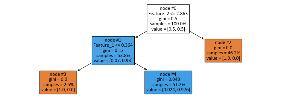
The following figure was generated utilizing dtreeviz.
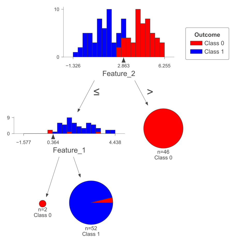
Fig. 10.8 Visual representation of the above Decision Tree Classifier.#
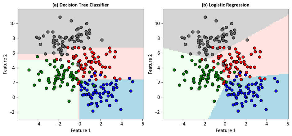
10.4.6. Example - Multiclass Classification#
Example - Multiclass Classification: Unlike our earlier binary classification focus, where we concentrated on just two classes, our current journey involves untangling the complexities of categorizing across a multitude of distinct classes.
import numpy as np
from sklearn.tree import DecisionTreeClassifier
from matplotlib.colors import ListedColormap
from sklearn.inspection import DecisionBoundaryDisplay

# Define colors and colormap for the plot
colors = ["Red", "Blue", "Green", 'DimGray']
cmap_light = ListedColormap(["MistyRose", "LightBlue", "HoneyDew", "LightGray"])

# Generate synthetic data using make_blobs
n_samples = 250
n_features = 2
centers = 4
cluster_std = 1.25
X, y = make_blobs(n_samples=n_samples, n_features=n_features, centers=centers, random_state=0, cluster_std=cluster_std)

# Create subplots for decision boundary visualization
fig, axes = plt.subplots(1, 2, figsize=(9.5, 4.5))
axes = axes.ravel()

# Define classifier models, names, and codes
models = [DecisionTreeClassifier(**{'max_features': 3, 'max_leaf_nodes': 10}),
          LogisticRegression(penalty='l2')]
model_names = ['Decision Tree Classifier', 'Logistic Regression']
model_codes = 'abcd'

# Loop through each classifier
for ax, classifier, name, code in zip(axes, models, model_names, model_codes):
    # Fit the classifier to the data
    classifier.fit(X, y)

    # Plot decision boundary using DecisionBoundaryDisplay
    DecisionBoundaryDisplay.from_estimator(classifier, X, cmap=cmap_light, ax=ax,
                                           response_method="predict",
                                           plot_method="pcolormesh",
                                           xlabel='Feature 1', ylabel='Feature 2',
                                           shading="auto")

    # Scatter plot for data points
    for num in np.unique(y):
        ax.scatter(X[:, 0][y == num], X[:, 1][y == num], c=colors[num],
                   s=40, edgecolors='k', marker='o', label=str(num))

    # Set title and remove grid lines
    ax.set_title(f'({code}) {name}', weight='bold')
    ax.grid(False)

# Adjust layout for better visualization
plt.tight_layout()
import numpy as np
import pandas as pd
from sklearn.model_selection import StratifiedKFold
from sklearn import metrics
from sklearn.tree import DecisionTreeClassifier
from sklearn.linear_model import LogisticRegression

# Function to print a line of underscores for separation
def _Line(n = 60, c = '_'):
    print(n * c)

def print_bold(txt, c = 32):
    print(f"\033[1;{c}m" + txt + "\033[0m")

# Sample data X and y are assumed to be defined here

# Models to be evaluated
model_alphs = 'ab'

# Loop through each model
for model, name, alph in zip(models, model_names, model_alphs):
    _Line(n = 80, c = '=')
    print_bold(f'({alph}) {name}', c = 35)
    _Line(n = 80, c = '=')

    # Initialize KFold cross-validator
    n_splits = 5
    skf = StratifiedKFold(n_splits=n_splits, shuffle=True, random_state=42)
    # The splitt would be 80-20!

    # Lists to store train and test scores for each fold
    train_acc_scores, test_acc_scores, train_f1_scores, test_f1_scores = [], [], [], []
    train_class_proportions, test_class_proportions = [], []

    # DataFrames to store classification reports
    reports_train = pd.DataFrame()
    reports_test = pd.DataFrame()

    # Perform Cross-Validation
    for fold, (train_idx, test_idx) in enumerate(skf.split(X, y), 1):
        X_train, X_test = X[train_idx], X[test_idx]
        y_train, y_test = y[train_idx], y[test_idx]
        model.fit(X_train, y_train)

        # Calculate class proportions for train and test sets
        train_class_proportions.append([np.mean(y_train == model) for model in np.unique(y)])
        test_class_proportions.append([np.mean(y_test == model) for model in np.unique(y)])

        # train
        y_train_pred = model.predict(X_train)
        train_acc_scores.append(metrics.accuracy_score(y_train, y_train_pred))
        train_f1_scores.append(metrics.f1_score(y_train, y_train_pred, average = 'weighted'))

        # test
        y_test_pred = model.predict(X_test)
        test_acc_scores.append(metrics.accuracy_score(y_test, y_test_pred))
        test_f1_scores.append(metrics.f1_score(y_test, y_test_pred, average = 'weighted'))

    _Line()
    #  Print the Train and Test Scores for each fold
    for fold in range(n_splits):
        print_bold(f'Fold {fold + 1}:')
        print(f"\tTrain Class Proportions: {train_class_proportions[fold]}*{len(y_train)}")
        print(f"\tTest Class Proportions: {test_class_proportions[fold]}*{len(y_test)}")
        print(f"\tTrain Accuracy Score = {train_acc_scores[fold]:.4f}, Test Accuracy Score = {test_acc_scores[fold]:.4f}")
        print(f"\tTrain F1 Score (weighted) = {train_f1_scores[fold]:.4f}, Test F1 Score (weighted)= {test_f1_scores[fold]:.4f}")

    _Line()
    print_bold('Accuracy Score:')
    print(f"\tMean Train Accuracy Score: {np.mean(train_acc_scores):.4f} ± {np.std(train_acc_scores):.4f}")
    print(f"\tMean Test Accuracy Score: {np.mean(test_acc_scores):.4f} ± {np.std(test_acc_scores):.4f}")
    print_bold('F1 Score:')
    print(f"\tMean F1 Accuracy Score (weighted): {np.mean(train_f1_scores):.4f} ± {np.std(train_f1_scores):.4f}")
    print(f"\tMean F1 Accuracy Score (weighted): {np.mean(test_f1_scores):.4f} ± {np.std(test_f1_scores):.4f}")
    _Line()
================================================================================
(a) Decision Tree Classifier
================================================================================
____________________________________________________________
Fold 1:
	Train Class Proportions: [0.255, 0.25, 0.245, 0.25]*200
	Test Class Proportions: [0.24, 0.26, 0.26, 0.24]*50
	Train Accuracy Score = 0.9550, Test Accuracy Score = 0.8400
	Train F1 Score (weighted) = 0.9553, Test F1 Score (weighted)= 0.8382
Fold 2:
	Train Class Proportions: [0.255, 0.25, 0.245, 0.25]*200
	Test Class Proportions: [0.24, 0.26, 0.26, 0.24]*50
	Train Accuracy Score = 0.9300, Test Accuracy Score = 0.8800
	Train F1 Score (weighted) = 0.9310, Test F1 Score (weighted)= 0.8859
Fold 3:
	Train Class Proportions: [0.25, 0.255, 0.25, 0.245]*200
	Test Class Proportions: [0.26, 0.24, 0.24, 0.26]*50
	Train Accuracy Score = 0.9600, Test Accuracy Score = 0.8000
	Train F1 Score (weighted) = 0.9600, Test F1 Score (weighted)= 0.8022
Fold 4:
	Train Class Proportions: [0.25, 0.255, 0.25, 0.245]*200
	Test Class Proportions: [0.26, 0.24, 0.24, 0.26]*50
	Train Accuracy Score = 0.9400, Test Accuracy Score = 0.9000
	Train F1 Score (weighted) = 0.9394, Test F1 Score (weighted)= 0.8968
Fold 5:
	Train Class Proportions: [0.25, 0.25, 0.25, 0.25]*200
	Test Class Proportions: [0.26, 0.26, 0.24, 0.24]*50
	Train Accuracy Score = 0.9250, Test Accuracy Score = 0.9200
	Train F1 Score (weighted) = 0.9252, Test F1 Score (weighted)= 0.9199
____________________________________________________________
Accuracy Score:
	Mean Train Accuracy Score: 0.9420 ± 0.0136
	Mean Test Accuracy Score: 0.8680 ± 0.0431
F1 Score:
	Mean F1 Accuracy Score (weighted): 0.9422 ± 0.0135
	Mean F1 Accuracy Score (weighted): 0.8686 ± 0.0426
____________________________________________________________
================================================================================
(b) Logistic Regression
================================================================================
____________________________________________________________
Fold 1:
	Train Class Proportions: [0.255, 0.25, 0.245, 0.25]*200
	Test Class Proportions: [0.24, 0.26, 0.26, 0.24]*50
	Train Accuracy Score = 0.9150, Test Accuracy Score = 0.8600
	Train F1 Score (weighted) = 0.9149, Test F1 Score (weighted)= 0.8614
Fold 2:
	Train Class Proportions: [0.255, 0.25, 0.245, 0.25]*200
	Test Class Proportions: [0.24, 0.26, 0.26, 0.24]*50
	Train Accuracy Score = 0.9050, Test Accuracy Score = 0.9000
	Train F1 Score (weighted) = 0.9041, Test F1 Score (weighted)= 0.9010
Fold 3:
	Train Class Proportions: [0.25, 0.255, 0.25, 0.245]*200
	Test Class Proportions: [0.26, 0.24, 0.24, 0.26]*50
	Train Accuracy Score = 0.9200, Test Accuracy Score = 0.8200
	Train F1 Score (weighted) = 0.9201, Test F1 Score (weighted)= 0.8143
Fold 4:
	Train Class Proportions: [0.25, 0.255, 0.25, 0.245]*200
	Test Class Proportions: [0.26, 0.24, 0.24, 0.26]*50
	Train Accuracy Score = 0.8950, Test Accuracy Score = 0.9200
	Train F1 Score (weighted) = 0.8943, Test F1 Score (weighted)= 0.9207
Fold 5:
	Train Class Proportions: [0.25, 0.25, 0.25, 0.25]*200
	Test Class Proportions: [0.26, 0.26, 0.24, 0.24]*50
	Train Accuracy Score = 0.8850, Test Accuracy Score = 0.9400
	Train F1 Score (weighted) = 0.8844, Test F1 Score (weighted)= 0.9397
____________________________________________________________
Accuracy Score:
	Mean Train Accuracy Score: 0.9040 ± 0.0128
	Mean Test Accuracy Score: 0.8880 ± 0.0431
F1 Score:
	Mean F1 Accuracy Score (weighted): 0.9036 ± 0.0131
	Mean F1 Accuracy Score (weighted): 0.8874 ± 0.0449
____________________________________________________________
from sklearn import tree
print('Models:', models)
dts = models[0]
dts.fit(X_train, y_train)

fig, ax = plt.subplots(1, 1, figsize=(16.5, 8))
_ = tree.plot_tree(dts, ax = ax,
                   filled = True,
                   node_ids = True,
                   feature_names = [f'Feature_{i + 1}' for i in range(2)],
                   proportion = True,
                   fontsize = 12)
plt.tight_layout()
Models: [DecisionTreeClassifier(max_features=3, max_leaf_nodes=10), LogisticRegression()]
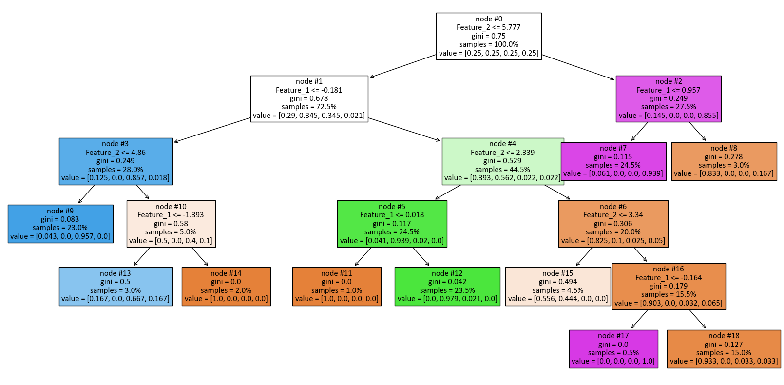
print(tree.export_text(dts, feature_names = [f'Feature_{i + 1}' for i in range(2)]))
|--- Feature_2 <= 5.78
|   |--- Feature_1 <= -0.18
|   |   |--- Feature_2 <= 4.86
|   |   |   |--- class: 2
|   |   |--- Feature_2 >  4.86
|   |   |   |--- Feature_1 <= -1.39
|   |   |   |   |--- class: 2
|   |   |   |--- Feature_1 >  -1.39
|   |   |   |   |--- class: 0
|   |--- Feature_1 >  -0.18
|   |   |--- Feature_2 <= 2.34
|   |   |   |--- Feature_1 <= 0.02
|   |   |   |   |--- class: 0
|   |   |   |--- Feature_1 >  0.02
|   |   |   |   |--- class: 1
|   |   |--- Feature_2 >  2.34
|   |   |   |--- Feature_2 <= 3.34
|   |   |   |   |--- class: 0
|   |   |   |--- Feature_2 >  3.34
|   |   |   |   |--- Feature_1 <= -0.16
|   |   |   |   |   |--- class: 3
|   |   |   |   |--- Feature_1 >  -0.16
|   |   |   |   |   |--- class: 0
|--- Feature_2 >  5.78
|   |--- Feature_1 <= 0.96
|   |   |--- class: 3
|   |--- Feature_1 >  0.96
|   |   |--- class: 0
10.4.7. Choosing Between Regression Trees and Linear Models#
The decision to use either Regression Trees or Linear Models depends on various factors related to your data’s characteristics, the underlying relationships you intend to model, and your overall objectives. Both Regression Trees and Linear Models possess distinct strengths and limitations, making the optimal choice contingent on your specific use case [Carrizosa et al., 2021, Efron and Hastie, 2021, scikit-learn Developers, 2023].
10.4.7.1. Regression Trees:#
Strengths:
Handling Non-Linearity: Regression Trees excel at capturing intricate, non-linear relationships in your data. They can uncover patterns that Linear Models may struggle to identify.
Automatic Feature Selection: Trees can handle a mix of numerical and categorical features, autonomously selecting relevant ones without extensive preprocessing efforts.
Interpretability: Trees are visually intuitive and offer transparent interpretations, aiding in explaining the decision-making process to stakeholders.
Outlier Robustness: Regression Trees tend to be less affected by outliers compared to certain linear models.
Weaknesses:
Overfitting Risk: Due to their potential to adapt closely to training data, Regression Trees can overfit, yielding suboptimal generalization on unseen data.
Sensitivity to Data Fluctuations: Minor changes in input data can lead to substantially different tree structures, making them sensitive to data variations.
Extrapolation Limitation: Regression Trees may not reliably predict values outside the range of training data.
10.4.7.2. Linear Models:#
Strengths:
Simplicity and Interpretability: Linear Models offer straightforward interpretations, particularly when relationships between variables are nearly linear.
Stability and Generalization: In scenarios involving small datasets or concerns about overfitting, Linear Models often yield more stable and better generalizable results.
Extrapolation Capability: Linear Models can predict values beyond the training data’s range, assuming the linear relationship persists.
Weaknesses:
Limited Non-Linearity: Linear Models might struggle to accurately model complex non-linear relationships inherent in the data.
Feature Engineering Demand: Capturing interactions and non-linearities in Linear Models may necessitate meticulous feature engineering.
Assumption of Linearity: Linear Models assume the relationship between predictors and the target variable is linear, which may not hold universally.
10.4.7.3. Choosing Between Them:#
Selecting the appropriate model hinges on your specific requirements:
Relationship Complexity: Opt for Regression Trees if non-linear relationships are suspected and you possess ample data.
Interpretation Priority: When clarity in explaining the model’s decisions is paramount, Regression Trees offer transparent insights.
Generalization Concerns: For scenarios involving concerns about overfitting or small datasets, Linear Models generally yield superior generalization.
Data Preparation: If extensive feature engineering is tolerable, Linear Models can be fine-tuned to handle interactions and non-linearities.
In practice, experimenting with both methods and evaluating their performance using techniques like cross-validation can be beneficial. Ensemble methods, such as Random Forests or Gradient Boosting Trees, merge the advantages of both Regression Trees and Linear Models, potentially delivering enhanced predictive outcomes. Ultimately, the model choice should be influenced by your unique data characteristics, problem domain, and overarching goals.