4.5. Applied Spatial Analysis Workflows

4.5.1. Learning objectives

By the end of this section, you should be able to:

• plan a spatial analysis as an auditable sequence of operations;

• name the unit of analysis and track how each stage changes what a row means;

• combine measurements, buffers, joins, and overlays in one workflow;

• distinguish coverage share, covered units, and distance to service as separate measures;

• quantify coverage and identify coverage gaps; and

• summarize findings with a map and a table that can be checked, stating the threshold and the limitations.

Section goal

Apply the S01–S04 building blocks end to end on two Calgary questions: how park sites are distributed across community districts, and how well libraries serve the districts as Euclidean coverage. Each workflow states its unit of analysis and validates every stage.

4.5.2. Plan the analysis before coding

An applied analysis is a chain of operations, and each link can change the answer without raising an error. Two habits keep the chain auditable: name the unit of analysis, and check every stage.

The unit of analysis is the thing that one row of the final table describes, here a community district. Every stage changes what a row means, which is its grain. Sampled parks have one row per park, a spatial join gives one row per park–district pair, an overlay gives one row per piece, and a summary gives one row per district. Count both the rows and the distinct units after each stage, because the two can move in opposite directions: fan-out raises the rows while a silent drop lowers the distinct units. Table 4.18 lists what to check at each kind of stage.

Table 4.18 What can go wrong at each stage of a workflow, and the check that catches it.

Stage	What can go wrong	Check
Load and parse	Swapped coordinates, missing geometry	Bounds, CRS, notna
Reproject	Areas or distances taken in degrees	Equal CRSs, projected units
Repair	Invalid rings break joins and overlays	is_valid.all() after make_valid
Join	Fan-out, unmatched rows	Rows against left rows, duplicated identifiers, null right columns
Overlay	Units dropped, slivers, wrong areas	Distinct units, area identities, smallest pieces
Buffer and dissolve	Distance in the wrong units, overlapping zones	Radius in metres, hand-checked area
Summary merge	Districts lost or duplicated	validate='one_to_one', row count

The toy example chains the stages of Workflow A on three parks and two districts and logs the grain after each stage. Park P1 lies in district D1, P2 straddles D1 and D2, and P3 lies outside both.

Show code cell source

Hide code cell source

import geopandas as gpd
import pandas as pd
from shapely.geometry import box

# Toy layers in metres.
districts = gpd.GeoDataFrame(
    {'district': ['D1', 'D2']},
    geometry=[box(0, 0, 100, 100), box(100, 0, 200, 100)],
)
parks = gpd.GeoDataFrame(
    {'park': ['P1', 'P2', 'P3']},
    geometry=[box(10, 10, 40, 40), box(80, 20, 120, 60), box(250, 0, 280, 30)],
)

log = []


def record(stage, rows, units, area):
    log.append({'stage': stage, 'rows': rows, 'distinct units': units, 'area (m²)': area})


record('parks', len(parks), parks['park'].nunique(), parks.area.sum())

joined = gpd.sjoin(parks, districts, how='left', predicate='intersects')
record('join (intersects)', len(joined), joined['park'].nunique(), joined.area.sum())
print('unmatched parks after the join:', int(joined['district'].isna().sum()))

pieces = gpd.overlay(parks, districts, how='intersection')
record('overlay (intersection)', len(pieces), pieces['park'].nunique(), pieces.area.sum())

summary = (
    pieces.assign(area_m2=pieces.area)
    .groupby('district')
    .agg(parks=('park', 'nunique'), park_area_m2=('area_m2', 'sum'))
    .reset_index()
)
record('district summary', len(summary), summary['district'].nunique(), summary['park_area_m2'].sum())

display(pd.DataFrame(log))
display(summary)

unmatched parks after the join: 1

	stage	rows	distinct units	area (m²)
0	parks	3	3	3400.0
1	join (intersects)	4	3	5000.0
2	overlay (intersection)	3	2	2500.0
3	district summary	2	2	2500.0

	district	parks	park_area_m2
0	D1	2	1700.0
1	D2	1	800.0

Read the log from top to bottom. The join raises the rows from 3 to 4 because P2 matches two districts, yet it keeps all 3 parks and reports P3 as unmatched. The overlay then drops P3 without a message, because P3 has no intersection to return, so the distinct parks fall to 2 and the area falls from 3,400 to 2,500 m². The area after the join is 5,000 m², more than the parks really cover, because a left join repeats P2’s whole geometry for each match. None of this is an error, and none of it is visible unless the log is printed. The Calgary workflows below repeat the pattern: state the unit, then print counts and totals at each stage.

4.5.3. Workflow A: park distribution across community districts

Question. Which community districts contain the most park area, and which sampled park sites cross district boundaries?

Plan. The unit of analysis is the community district. Load parks, districts, and the city boundary [Open Calgary: The City of Calgary Open Data Portal, 2026]; validate geometry; reproject to a metric CRS; join park sites to districts spatially; overlay to measure the shared area; then summarize per district. Table 4.19 lists the steps and where each is covered.

Table 4.19 Workflow A steps, the operation used at each, and the section that covers it.

Step	Operation	Section
Load and parse layers	read_file, from_wkt	S01
Validate types, CRS, validity	inspection assertions	S01, S06
Metric measurements	to_crs, area	S02
Assign parks to districts	sjoin with intersects	S03
Split shared areas	overlay intersection	S04
Summarize per district	groupby, merge	S03

One district polygon has a self-intersecting ring, so the workflow repairs it explicitly before the join and overlay stages; S06 covers this pattern in detail.

Show code cell source

Hide code cell source

from pathlib import Path

import geopandas as gpd
import pandas as pd

DATA_DIR = Path('../data') if Path('../data').exists() else Path('data')

parks = gpd.read_file(DATA_DIR / 'Parks_Sites_20261019.geojson')
parks = (
    parks.loc[parks.geometry.notna()]
    .sort_values('asset_cd', kind='stable')
    .head(300)
    .copy()
)

communities_raw = pd.read_csv(DATA_DIR / 'Community_District_Boundaries_20240620.csv')
communities = gpd.GeoDataFrame(
    communities_raw,
    geometry=gpd.GeoSeries.from_wkt(communities_raw['MULTIPOLYGON']),
    crs='EPSG:4326',
)

city_boundary = gpd.read_file(DATA_DIR / 'City Boundary_20240620.gpkg')

metric_crs = parks.estimate_utm_crs()
parks_m = parks.to_crs(metric_crs)
communities_m = communities.to_crs(metric_crs)
city_m = city_boundary.to_crs(metric_crs)

# Stage validation: CRS alignment, geometry presence, and validity.
assert parks_m.crs == communities_m.crs == city_m.crs
assert parks_m.geometry.notna().all() and communities_m.geometry.notna().all()

# One district ring self-intersects. Repair it explicitly rather than dropping the
# feature, and confirm the layer is fully valid before joining or overlaying.
from shapely.validation import make_valid

communities_m['geometry'] = communities_m.geometry.map(make_valid)
assert parks_m.geometry.is_valid.all()
assert communities_m.geometry.is_valid.all()
print('layers aligned on', metric_crs)

layers aligned on EPSG:32611

4.5.3.1. Assign parks to districts

Both layers are polygons, so the predicate decides what counts as belonging. within keeps only parks that lie entirely inside one district and silently loses every park that straddles a boundary. intersects keeps every park that touches a district and returns one row per district it touches. This workflow needs to see the boundary-crossing parks, so it uses intersects and expects more rows than parks, as in S03.

The spatial join attaches each park site to the district containing it. Reporting the unmatched count keeps boundary cases visible instead of letting them disappear.

Show code cell source

Hide code cell source

park_assignment = gpd.sjoin(
    parks_m[['asset_cd', 'site_name', 'geometry']],
    communities_m[['COMM_CODE', 'NAME', 'geometry']],
    how='left',
    predicate='intersects',
)

print('sampled parks:', len(parks_m))
print('assignment rows:', len(park_assignment))
print('parks crossing district boundaries:',
      int(park_assignment['asset_cd'].duplicated().sum()))
print('parks outside every district:',
      int(park_assignment['COMM_CODE'].isna().sum()))

sampled parks: 300
assignment rows: 334
parks crossing district boundaries: 34
parks outside every district: 1

The join returns 334 rows for 300 parks. The printed 34 counts the extra rows, not the parks: a park that touches three districts adds two. The number of distinct parks that match more than one district can be smaller, and it also includes parks that only touch a boundary, which the overlay below turns into zero-area pieces. The index of the left layer identifies each park, so counting its repeats gives the park-level answer.

Show code cell source

Hide code cell source

matches_per_park = park_assignment.index.value_counts()
print('extra rows created by the join:', len(park_assignment) - len(parks_m))
print('distinct parks matching more than one district:', int((matches_per_park > 1).sum()))

extra rows created by the join: 34
distinct parks matching more than one district: 27

4.5.3.2. Measure shared areas with an overlay

The join says which district a park touches; the overlay says how much of each park lies in each district. Totals per district must stay below the sampled park area, and the identifiers let every piece be traced back to its source.

Show code cell source

Hide code cell source

park_pieces = gpd.overlay(
    parks_m[['asset_cd', 'site_name', 'geometry']],
    communities_m[['COMM_CODE', 'NAME', 'geometry']],
    how='intersection',
    keep_geom_type=False,
)
park_pieces['shared_area_ha'] = park_pieces.geometry.area / 10_000

district_summary = (
    park_pieces.groupby(['COMM_CODE', 'NAME'])
    .agg(
        park_sites=('asset_cd', 'nunique'),
        park_area_ha=('shared_area_ha', 'sum'),
    )
    .reset_index()
)
districts_with_parks = communities_m.merge(
    district_summary, on=['COMM_CODE', 'NAME'], how='left', validate='one_to_one'
)
districts_with_parks[['park_sites', 'park_area_ha']] = (
    districts_with_parks[['park_sites', 'park_area_ha']].fillna(0)
)

print(district_summary.sort_values('park_area_ha', ascending=False).head())
assert len(districts_with_parks) == len(communities_m)
assert district_summary['park_area_ha'].sum() <= parks_m.geometry.area.sum() / 10_000

   COMM_CODE                          NAME  park_sites  park_area_ha
7        12B                           12B           3    276.427256
10       ABP          AURORA BUSINESS PARK           2     76.060064
16       ARB                   ARBOUR LAKE          29     73.192695
27       BOW                       BOWNESS          36     68.587938
12       ALB  ALBERT PARK/RADISSON HEIGHTS          10     67.701764

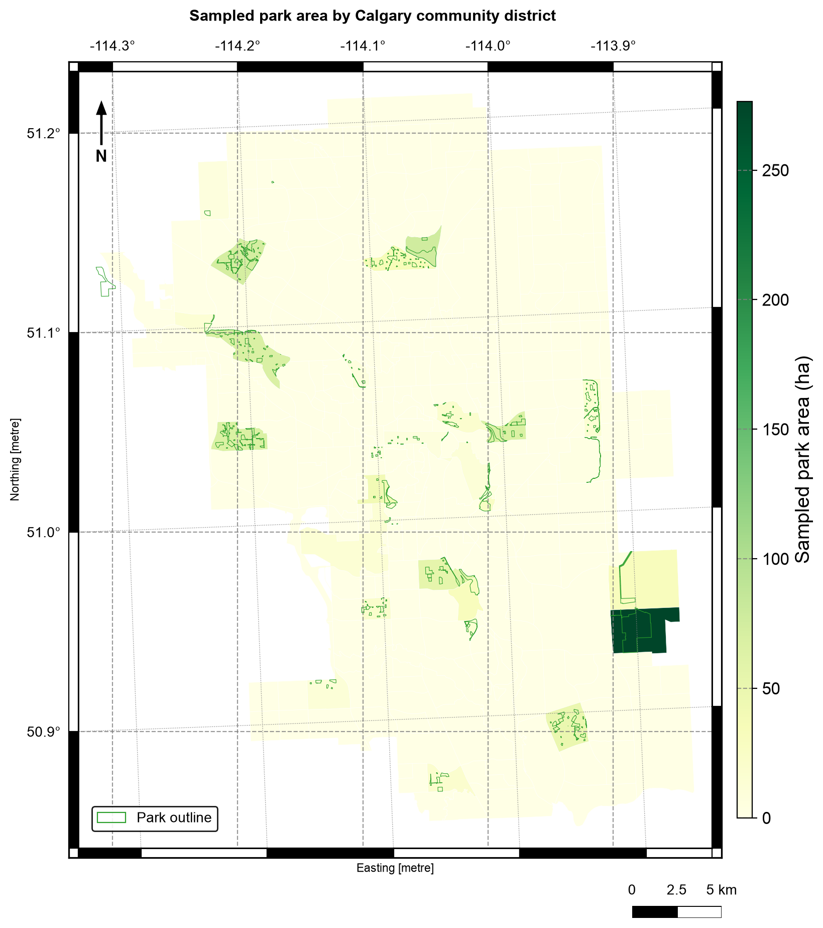
Fig. 4.9 Sampled park area (hectares) by Calgary community district, with the sampled park outlines in green. Data: City of Calgary Open Data.

In Fig. 4.9, district 12B on the eastern edge holds about 276 ha, more than three times the next district (Aurora Business Park, 76 ha), so it takes the top of the colour scale and most other districts look pale. Count and area also tell different stories: 12B has only three park sites, while Bowness has 36 sites but only 69 ha. The districts with park area are clustered because the sample is the first 300 parks by asset code, as in S04. District totals also depend on where the boundaries are drawn, a general limitation of area summaries known as the modifiable areal unit problem [Fotheringham and Wong, 1991, Openshaw, 1983].

Read the table with its unit in mind. park_sites counts distinct parks within each district, so a park that crosses a boundary is counted once in every district it touches. Adding the district counts therefore overstates the number of parks, exactly as in the double-counting example in S03. The overlay also drops the one park that lies outside every district, which is why the join reported it as unmatched and the district table does not contain it.

4.5.4. Workflow B: library coverage and gaps

Question. Which districts lie within a 500-metre Euclidean service zone of a library, and which have no library at all?

Plan. The unit of analysis is again the community district. Buffer the library points in a metric CRS, dissolve the buffers into one coverage geometry, then use an overlay to compare coverage against the district layer. A district with no library is not the same as a district outside the coverage zone — the two results answer different questions and are reported separately.

4.5.4.1. Three ways to measure coverage

“How well are districts served?” is several questions, and each needs its own measure [Geurs and Van Wee, 2004]. Table 4.20 separates them so that results are not mixed up.

Table 4.20 Coverage measures, the operation behind each, and its limitation.

Measure	Question it answers	Operation	Limitation
Coverage share	What fraction of the city lies within 500 m of a library?	buffer, union_all, area ratio	Ignores where people live
Covered districts	Which districts have a representative point inside a zone?	sjoin with within	One point stands in for a whole district
Distance to service	How far is each district from its nearest library?	sjoin_nearest	Straight-line, not a route
Gap area	Where is no service available?	difference overlay	Depends entirely on the threshold distance

Dissolving the buffers into one geometry means a point can match at most one coverage feature, which keeps the covered flag to one value per district.

Show code cell source

Hide code cell source

def location_to_point(value):
    '''Convert Calgary '(latitude, longitude)' text to a Point.'''
    from shapely.geometry import Point
    parts = [float(part.strip()) for part in value.strip('() ').split(',')]
    if len(parts) != 2:
        raise ValueError(f'Expected latitude and longitude, got: {value!r}')
    latitude, longitude = parts
    if not 49 <= latitude <= 53 or not -117 <= longitude <= -111:
        raise ValueError(f'Unexpected Calgary coordinate order or range: {value!r}')
    return Point(longitude, latitude)


libraries_raw = pd.read_csv(DATA_DIR / 'Calgary_Public_Library_Locations_and_Hours_20240620.csv')
libraries = gpd.GeoDataFrame(
    libraries_raw,
    geometry=libraries_raw['Location'].map(location_to_point),
    crs='EPSG:4326',
).reset_index(names='branch_id')
libraries_m = libraries.to_crs(metric_crs)

coverage = gpd.GeoDataFrame(geometry=[libraries_m.geometry.buffer(500).union_all()], crs=metric_crs)
coverage_area_km2 = coverage.geometry.area.sum() / 1_000_000
city_area_km2 = city_m.geometry.area.sum() / 1_000_000

print(f'combined 500 m coverage: {coverage_area_km2:.1f} km²')
print(f'city boundary area:      {city_area_km2:.1f} km²')
print(f'nominal coverage share:  {coverage_area_km2 / city_area_km2:.1%}')

combined 500 m coverage: 14.1 km²
city boundary area:      852.9 km²
nominal coverage share:  1.7%

A hand check supports the number. A 500 m buffer around one point covers about π × 0.5² ≈ 0.785 km², and 18 branches give roughly 14.1 km². That matches the combined coverage, so the buffers hardly overlap. The share is nominal: it divides the buffer area by the city area, even though buffers near the edge can extend past the boundary.

4.5.4.2. Distance to the nearest library

Buffer coverage is a binary inside/outside answer. A distance field keeps the gradation: districts whose representative point is far from any branch flag where a Euclidean service model is weakest. The representative point (S02) is used because it is guaranteed to fall inside its district, unlike a centroid. It stands in for the district in a screening distance and is not a population location.

Show code cell source

Hide code cell source

district_points = communities_m.copy()
district_points['geometry'] = communities_m.geometry.representative_point()

nearest = gpd.sjoin_nearest(
    district_points[['COMM_CODE', 'NAME', 'geometry']],
    libraries_m[['Library', 'geometry']],
    how='left',
    distance_col='distance_to_library_m',
)

covered_flags = (
    gpd.sjoin(
        district_points[['COMM_CODE', 'geometry']],
        coverage,
        how='left',
        predicate='within',
    )[['COMM_CODE', 'index_right']]
    .rename(columns={'index_right': 'coverage_id'})
    # One flag per district even if a boundary touches more than one match.
    .drop_duplicates(subset='COMM_CODE')
)

district_access = nearest.merge(covered_flags, on='COMM_CODE', validate='one_to_one')
district_access['within_500m'] = district_access['coverage_id'].notna()

print(district_access[['NAME', 'Library', 'distance_to_library_m', 'within_500m']]
      .sort_values('distance_to_library_m', ascending=False)
      .head(10))
print('district representative points within 500 m of a library:',
      int(district_access['within_500m'].sum()), 'of', len(district_access))
assert district_access['COMM_CODE'].is_unique

              NAME                  Library  distance_to_library_m  \
228            12L  Glenmore Square Library           12831.929758   
235            12J        Shawnessy Library           12808.745416   
240      HOTCHKISS  Glenmore Square Library           11278.563521   
225      RANGEVIEW        Shawnessy Library           10444.122530   
233            12C  Glenmore Square Library           10129.055787   
239  RICARDO RANCH        Shawnessy Library           10065.325786   
238    COPPERFIELD  Glenmore Square Library            9881.871894   
237       MAHOGANY        Shawnessy Library            9729.607290   
287            13A        Southwood Library            9625.960872   
278            13E        Shawnessy Library            9526.009673   

     within_500m  
228        False  
235        False  
240        False  
225        False  
233        False  
239        False  
238        False  
237        False  
287        False  
278        False  
district representative points within 500 m of a library: 5 of 313

Only 5 of the 313 district representative points are within 500 m of a library (1.6%), close to the 1.7% area share, but the two measures count different things: one point per district against the share of the city’s area. The ten districts farthest from a branch all have Glenmore Square, Shawnessy, or Southwood as their nearest library, at distances of 9.5 to 12.8 km, so the largest distances lie toward the southern edge of the city. A district’s nearest library is only the nearest in a straight line.

4.5.4.3. Identify coverage gaps

The gap layer is the city minus the coverage geometry — a difference overlay. Gaps inside the boundary matter; areas outside it do not. Clipping the gap to the city boundary keeps the map and the area totals honest.

This is the difference identity from S04: the area of the city equals the area of the coverage inside it plus the area of the gap. The assertion in the next cell checks that identity within a 1% tolerance.

Show code cell source

Hide code cell source

gap = gpd.overlay(city_m[['geometry']], coverage, how='difference', keep_geom_type=False)
gap_area_km2 = gap.geometry.area.sum() / 1_000_000

print(f'coverage gap inside the city: {gap_area_km2:.1f} km²')
# Coverage plus gap must reconstruct the city area (within rounding).
assert abs((coverage.clip(city_m).geometry.area.sum() + gap.geometry.area.sum())
           - city_m.geometry.area.sum()) < city_m.geometry.area.sum() * 0.01

coverage gap inside the city: 838.7 km²

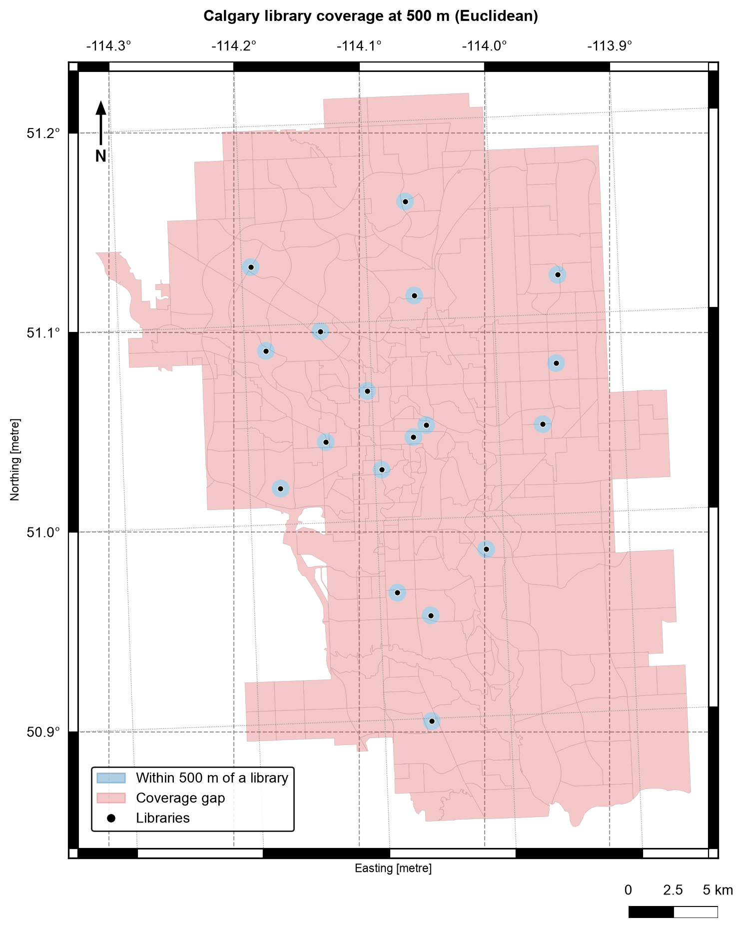
Fig. 4.10 Calgary library coverage at 500 m (Euclidean): the zone within 500 m of a library (blue) and the coverage gap (red), with district boundaries in grey.

Fig. 4.10 shows how little of the city a 500 m zone reaches: the 18 small blue disks sit inside a red gap that covers 838.7 km² of the 852.9 km² city, about 98.3%. The disks hardly overlap, which matches the hand check above. The map says nothing about whether 500 m is the right distance, which is why the threshold test below matters.

4.5.4.4. Test the threshold

The 500 m radius is a choice, not a fact, and every coverage number depends on it. A finding is more defensible when it shows how much the answer changes with the threshold.

Show code cell source

Hide code cell source

city_area = city_m.geometry.area.sum()
for radius in [250, 500, 1000, 2000]:
    zone_area = libraries_m.geometry.buffer(radius).union_all().area
    print(f'{radius:>5} m: {zone_area / city_area:.1%} nominal coverage')

  250 m: 0.4% nominal coverage
  500 m: 1.7% nominal coverage
 1000 m: 6.5% nominal coverage
 2000 m: 24.2% nominal coverage

Coverage grows quickly but not without limit: doubling the radius from 250 m to 500 m multiplies the nominal coverage by about four (0.4% to 1.7%), as buffer area scales with the square of the radius, but doubling from 1,000 m to 2,000 m multiplies it by only 3.7 (6.5% to 24.2%), because the zones begin to overlap. Even at 2 km, three quarters of the city lies outside every zone.

4.5.5. From results to findings

A defensible summary names the unit, the threshold, and the limitation:

• The park analysis reports sampled sites only; the 300-feature sample is for learning the workflow, not for a Calgary-wide park inventory.

• The coverage analysis uses Euclidean buffers, not walking routes. A district whose representative point is within 500 metres of a branch can still contain homes much farther away, and network distance is the subject of Chapter 5.

• Both workflows keep identifiers, print row counts, and assert invariants, so a reviewer can rerun the notebook and check every stage.

4.5.6. Summary

Complete analyses chain the chapter’s building blocks: parse and inspect (S01), measure and buffer in a projected CRS (S02), join with explicit cardinality (S03), and overlay to measure shared or excluded area (S04). Name the unit of analysis, track how each stage changes the grain, and print rows, distinct units, and areas so that fan-out, silent drops, and threshold effects are visible. Continue with S06 to make validation a habit rather than an afterthought.