4.2. Geometric Operations and Measurements

4.2.1. Learning objectives

By the end of this section, you should be able to:

• choose an operation from a spatial question;

• distinguish measurements from geometry transformations;

• explain why metric operations require a projected CRS;

• state what area, length, and distance report for each geometry type;

• derive envelopes, centroids, convex hulls, buffers, and representative points, and explain what each one means;

• simplify geometries and describe the trade-off;

• explain how a spatial index filters candidates, and compare a slow pairwise loop with an indexed spatial operation; and

• check units, geometry types, and plausible ranges after an operation.

Section goal

Use Calgary parks, libraries, and LRT tracks to calculate meaningful areas and lengths, then create proximity zones without confusing a Euclidean buffer with a network route.

4.2.2. Start with the question

Every operation in this section answers a specific kind of spatial question. Table 4.8 maps common questions to the GeoPandas [Jordahl et al., 2020] operation or property that answers them.

Table 4.8 Spatial questions and the GeoPandas operation or property that answers each.

Question	Operation or property
How large is each park?	area in a projected CRS
How long is each track segment?	length in a projected CRS
What is within 500 metres of a library?	buffer
What is the smallest box around a layer?	envelope / total_bounds
Where can a park be labelled?	representative_point
What is the smallest convex shape covering the libraries?	convex_hull
How can a layer be made lighter for display?	simplify

A transformation changes geometry; a measurement reports a property of a geometry. Both must be interpreted in the CRS units. In EPSG:4326, an area is in square degrees and a distance is in degrees, so those values are not suitable for metric reporting.

4.2.3. Why metric operations need a projected CRS

Every measurement inherits the units of the CRS, so the first decision in this section is which kind of CRS the coordinates use. Table 4.9 compares the two kinds.

Table 4.9 Geographic and projected coordinate reference systems.

Property	Geographic (for example EPSG:4326)	Projected (for example UTM)
Coordinates	Longitude and latitude on an ellipsoid	Easting and northing on a plane
Units	Degrees	Metres
Metric results	Not meaningful	Meaningful inside the zone it was designed for
Best for	Storage, exchange, web maps	Area, length, distance, buffers

A degree is not a constant length. A degree of latitude is about 111 km everywhere, but a degree of longitude shrinks with the cosine of the latitude, to roughly 70 km at Calgary. An area in square degrees, or a buffer(500) that means 500 degrees, therefore has no physical meaning, and GeoPandas warns when you ask for an area or length in a geographic CRS.

No flat map preserves everything. Each projection trades off area, shape, and distance, so the CRS should match the property you measure. UTM zones are conformal [Snyder, 1987], meaning they preserve local shape, and keep area and length errors small inside their six-degree zone. For a study spanning many zones, an equal-area projection is the better choice for areas. The cell below measures one 0.1 by 0.1 degree cell over Calgary both ways.

Show code cell source

Hide code cell source

import warnings

import geopandas as gpd
from pyproj import Geod
from shapely.geometry import box

# A 0.1 x 0.1 degree cell over Calgary.
cell = gpd.GeoSeries([box(-114.10, 51.00, -114.00, 51.10)], crs='EPSG:4326')
utm = cell.estimate_utm_crs()
cell_m = cell.to_crs(utm)

with warnings.catch_warnings():
    warnings.simplefilter('ignore')   # GeoPandas warns about area in a geographic CRS
    print('area in EPSG:4326:', round(cell.area.iloc[0], 4), 'square degrees')
print(f'area in {utm.name}: {cell_m.area.iloc[0] / 1e6:.1f} km²')

# The same 0.1 degree step is a different distance in each direction.
geod = Geod(ellps='WGS84')
east_west = geod.inv(-114.10, 51.05, -114.00, 51.05)[2]
north_south = geod.inv(-114.05, 51.00, -114.05, 51.10)[2]
print(f'0.1 degree east-west: {east_west / 1000:.1f} km, north-south: {north_south / 1000:.1f} km')

area in EPSG:4326: 0.01 square degrees
area in WGS 84 / UTM zone 11N: 78.0 km²
0.1 degree east-west: 7.0 km, north-south: 11.1 km

The same 0.1° cell is 0.01 square degrees or 78.0 km², and a 0.1° step spans 7.0 km east-west but 11.1 km north-south (geodesic distances on the WGS 84 ellipsoid [Karney, 2013]). A buffer of 0.1 degrees would therefore be an ellipse on the ground, not a circle.

4.2.4. Load the layers and choose an analysis CRS

The next cell loads the three layers [Open Calgary: The City of Calgary Open Data Portal, 2026] used in this section with the same parsing as S01 and creates metric copies, marked with the suffix _m, in a local UTM CRS. The source layers stay in EPSG:4326, so every measurement is derived from them and never overwrites them.

Show code cell source

Hide code cell source

from pathlib import Path

import geopandas as gpd
import pandas as pd
from shapely.geometry import Point

DATA_DIR = Path('../data') if Path('../data').exists() else Path('data')


def location_to_point(value):
    '''Convert Calgary '(latitude, longitude)' text to a Point.'''
    parts = [float(part.strip()) for part in value.strip('() ').split(',')]
    if len(parts) != 2:
        raise ValueError(f'Expected latitude and longitude, got: {value!r}')
    latitude, longitude = parts
    if not 49 <= latitude <= 53 or not -117 <= longitude <= -111:
        raise ValueError(f'Unexpected Calgary coordinate order or range: {value!r}')
    return Point(longitude, latitude)


parks = gpd.read_file(DATA_DIR / 'Parks_Sites_20261019.geojson')
libraries_raw = pd.read_csv(DATA_DIR / 'Calgary_Public_Library_Locations_and_Hours_20240620.csv')
libraries = gpd.GeoDataFrame(
    libraries_raw,
    geometry=libraries_raw['Location'].map(location_to_point),
    crs='EPSG:4326',
)
tracks_raw = pd.read_csv(DATA_DIR / 'Tracks_-_LRT_20240622.csv')
tracks = gpd.GeoDataFrame(
    tracks_raw,
    geometry=gpd.GeoSeries.from_wkt(tracks_raw['the_geom']),
    crs='EPSG:4326',
)

metric_crs = parks.estimate_utm_crs()
parks_m = parks.to_crs(metric_crs)
libraries_m = libraries.to_crs(metric_crs)
tracks_m = tracks.to_crs(metric_crs)

print('analysis CRS:', metric_crs)
print('park bounds in metres:', parks_m.total_bounds)

analysis CRS: EPSG:32611
park bounds in metres: [ 687584.38265866 5637217.70401382  719063.97072512 5675497.13094293]

4.2.5. What measurements report

A measurement returns a number for each geometry, and what that number means depends on the geometry type. Table 4.10 summarizes the three core measurements.

Table 4.10 What area, length, and distance report for each geometry type.

Measurement	Point	LineString	Polygon	Units
area	0	0	Enclosed area, minus holes	CRS units squared
length	0	Sum of segment lengths	Perimeter of every ring	CRS units
distance(other)	To the nearest part of other	Same	Same, and 0 if the two intersect	CRS units

Multipart geometries add up their parts. distance is the shortest straight-line gap between any two points of the geometries, not the gap to a centroid, and a point inside a polygon is 0 away from it. Measurements on an invalid geometry are unreliable: the bow-tie in S01 reports an area of zero, which is why the cell below checks the park geometries and repairs any invalid ones before measuring.

4.2.6. Measure in a projected CRS

estimate_utm_crs() chooses a local UTM CRS from the layer extent. For a regional or multi-country study, choose and document a CRS whose distortion properties fit the measurement instead. The values below are measurements of the source geometries, not new features.

The next cell checks validity after reprojection and repairs any invalid ring explicitly before measuring. In this download the check finds none: the one invalid geometry in S01 is a community district, not a park. make_valid returns a topologically valid geometry, possibly with a different part structure, so a repair can change a feature’s parts. See S06 for a fuller repair workflow.

Show code cell source

Hide code cell source

from shapely.validation import make_valid

parks_m = parks_m.copy()
tracks_m = tracks_m.copy()

invalid_metric = ~parks_m.geometry.is_valid
print('invalid park geometries after reprojection:', int(invalid_metric.sum()))
if invalid_metric.any():
    parks_m.loc[invalid_metric, 'geometry'] = (
        parks_m.loc[invalid_metric, 'geometry'].map(make_valid)
    )
assert parks_m.geometry.is_valid.all()

parks_m['area_ha'] = parks_m.geometry.area / 10_000
tracks_m['length_km'] = tracks_m.geometry.length / 1_000

print(parks_m[['site_name', 'area_ha']].head())
print(tracks_m['length_km'].describe())

assert (parks_m['area_ha'] >= 0).all()
assert (tracks_m['length_km'] >= 0).all()
assert parks_m.crs == tracks_m.crs == libraries_m.crs

invalid park geometries after reprojection: 0
                                           site_name    area_ha
0                                  OLD REFINERY PARK  26.936535
1                                     FAST FOOD PARK   0.485463
2                               CONSTABLE SLOPE PARK   1.718866
3                                       OUTWEST PARK   0.195589
4  FLUOR DANIELS PARK; RENFREW EDUCATIONAL SERVIC...   1.106836
count    5354.000000
mean        0.051735
std         0.231640
min         0.000473
25%         0.003101
50%         0.003101
75%         0.003101
max         2.745717
Name: length_km, dtype: float64

The track layer is highly fragmented. The three quartiles are all 3.1 m, so most of the 5,354 segments are only a few metres long, while the longest is 2.7 km and the mean is 52 m; together they sum to about 277 km. A count of segments therefore says nothing about network length, and length_km has to be summed. Park areas span a wide range too, from about 27 ha for Old Refinery Park to 0.2 ha for Outwest Park.

4.2.7. Simple derived geometries: envelopes, centroids, and convex hulls

A transformation returns a new geometry. Four simple derived geometries summarize a feature, each in a different way:

• the envelope is the smallest axis-aligned rectangle containing a feature, returned as a polygon, whereas bounds returns the same box as four numbers and total_bounds is the envelope of a whole layer;

• the centroid is the centre of mass of a polygon (the mean position for points and the length-weighted position for lines). It is a summary, not a guaranteed location: it falls outside a C-shaped polygon, a crescent, or a ring around a hole;

• the convex hull is the smallest convex shape containing a geometry or a collection of geometries, like a rubber band stretched around them. For any two points inside a convex shape, the straight line between them is inside too; and

• the representative point is a point guaranteed to lie on the feature, found by an algorithm rather than a formula. It is neither the centre nor unique, which makes it the safe choice for labels and for matching points to polygons.

All four trade detail for simplicity; use them for indexing, summaries, and display rather than as replacements for the source geometry. The C-shaped polygon below shows how they differ on one feature.

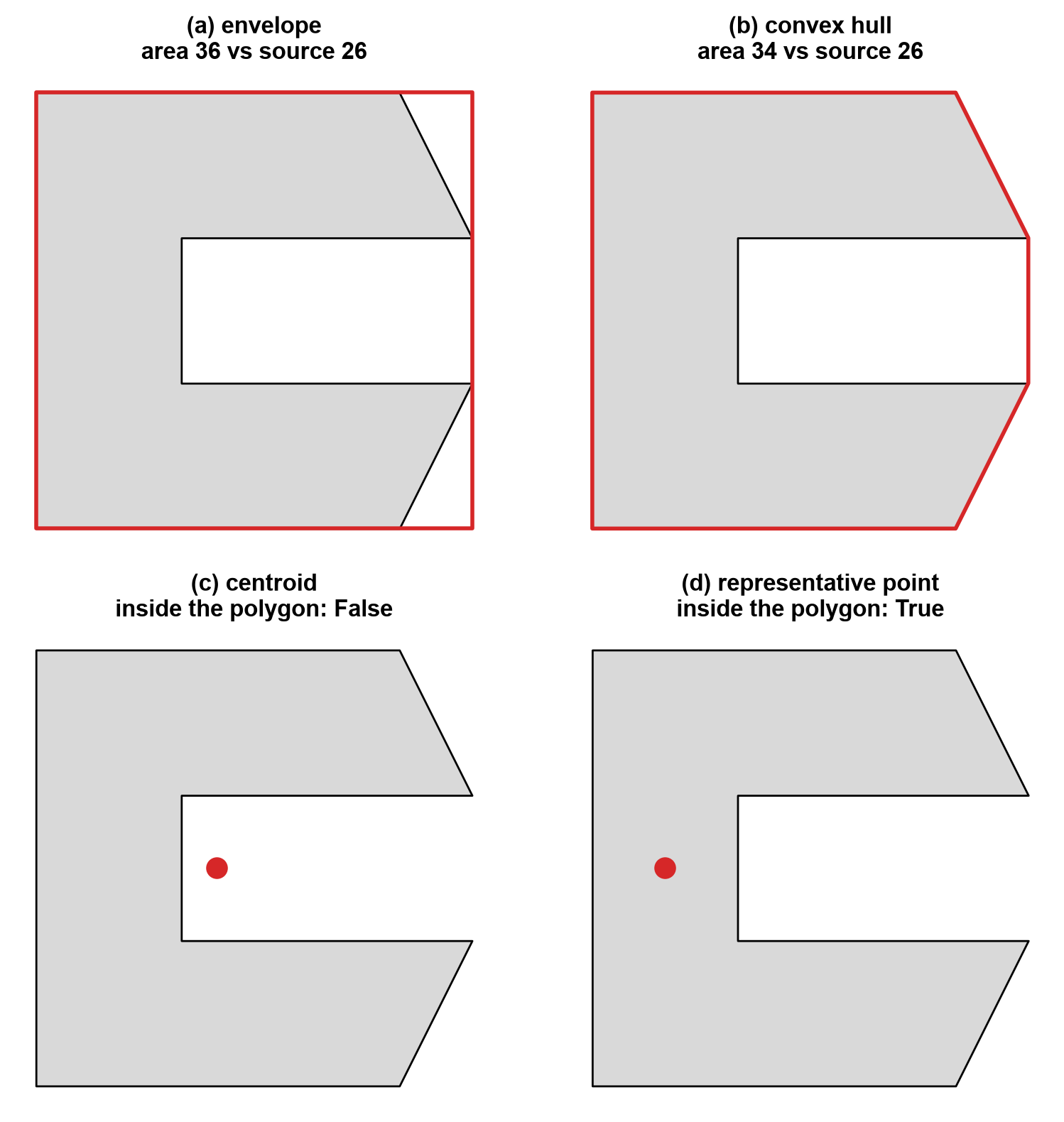
Fig. 4.3 Four derived geometries (red) of one C-shaped polygon: envelope, convex hull, centroid, and representative point.

In Fig. 4.3, the centroid lands in the notch, outside the polygon, while the representative point stays on the shape. The envelope and the hull both overstate the footprint (areas of 36 and 34 against 26 for the source), and the hull is the tighter of the two. The same operations on the Calgary layers:

Show code cell source

Hide code cell source

parks_m['envelope'] = parks_m.geometry.envelope
parks_m['centroid'] = parks_m.geometry.centroid
library_hull = libraries_m.union_all().convex_hull

print('layer extent (m):', parks_m.total_bounds.round(0))
print('envelope types:', parks_m['envelope'].geom_type.value_counts().to_dict())
print('centroid types:', parks_m['centroid'].geom_type.value_counts().to_dict())
print('convex hull of libraries:', library_hull.geom_type,
      f'{library_hull.area / 1_000_000:.1f} km²')

# A centroid can fall outside a concave polygon; count how often.
centroid_inside = parks_m['centroid'].within(parks_m.geometry).mean()
print(f'centroids inside their polygon: {centroid_inside:.1%}')

layer extent (m): [ 687584. 5637218.  719064. 5675497.]
envelope types: {'Polygon': 3036}
centroid types: {'Point': 3036}
convex hull of libraries: Polygon 309.9 km²
centroids inside their polygon: 91.6%

About 8% of the park centroids (91.6% fall inside) lie outside their own polygon, roughly one park in twelve, which is why the centroid is a summary and not a location. The convex hull of the 18 libraries encloses 309.9 km²; as a hull it says nothing about where the libraries are inside it.

4.2.8. Buffers and service zones

A buffer is the set of all points within a given distance of a geometry. The distance is in CRS units, so it must be metres from a projected CRS. Table 4.11 shows what a buffer produces for each input type.

Table 4.11 Buffer output by input geometry type.

Input	Buffer shape	Notes
Point	A circle, stored as a polygon	quad_segs sets segments per quarter circle (default 16, so 64 vertices)
LineString	A rounded corridor	cap_style and join_style control line ends and corners
Polygon	The outline pushed outward	A negative distance shrinks it, and can return an empty geometry

Because a circle is stored as a polygon, its area is a close approximation, not exact. dissolve() merges overlapping geometries into one row and aggregates their attributes, whereas union_all() returns a single Shapely geometry with no attributes.

Show code cell source

Hide code cell source

import math

from shapely.geometry import LineString, Point, Polygon

# Toy coordinates in metres.
site = Point(0, 0)
road = LineString([(0, 0), (800, 0), (800, 600)])
lot = Polygon([(0, 0), (800, 0), (800, 500), (0, 500)])

circle = site.buffer(500)
print('circle vertices:', len(circle.exterior.coords) - 1,
      '  area ratio to pi*r^2:', round(circle.area / (math.pi * 500 ** 2), 4))
print('lot buffered by -300 m is empty:', lot.buffer(-300).is_empty)

circle vertices: 64   area ratio to pi*r^2: 0.9984
lot buffered by -300 m is empty: True

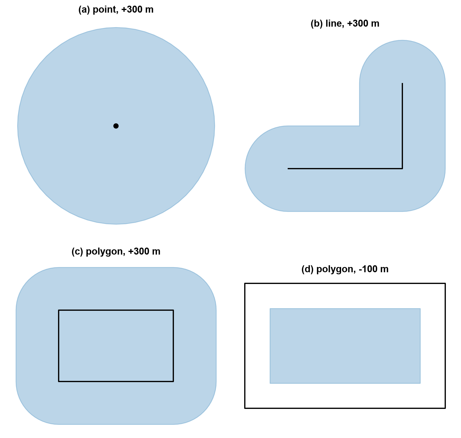
Fig. 4.4 Buffers of a point, a line, and a polygon (blue) around their sources (black), with a negative buffer on the polygon in panel (d).

Fig. 4.4 shows the shape each input produces: a circle for the point, a rounded corridor with round caps and a rounded outer corner for the line, and the polygon’s outline pushed outward with rounded corners. A negative distance (panel d) shrinks the polygon by 100 m on every side. The sign matters: the same lot shrunk by 300 m disappears, because its shorter side is 500 m and a 300 m inset needs 600 m. The 64-vertex circle covers 99.84% of the ideal area, a small, systematic underestimate.

4.2.8.1. Service zones around libraries

A 500-metre buffer answers “within 500 metres as the crow flies.” It does not answer “reachable within 500 metres along streets”; that question requires a network and a cost field (see Chapter 5). Dissolving the individual buffers creates one combined coverage geometry, while keeping them separate preserves the service zone for each library. The map after the checks overlays the zones on park outlines.

Show code cell source

Hide code cell source

library_buffers = libraries_m[['Library', 'geometry']].copy()
library_buffers['geometry'] = library_buffers.geometry.buffer(500)
combined_coverage = library_buffers.dissolve()

print('individual service zones:', len(library_buffers))
print('combined coverage geometries:', len(combined_coverage))
print('combined coverage area (km²):',
      combined_coverage.geometry.area.sum() / 1_000_000)

assert library_buffers.geometry.geom_type.isin(['Polygon', 'MultiPolygon']).all()
assert combined_coverage.geometry.notna().all()

individual service zones: 18
combined coverage geometries: 1
combined coverage area (km²): 14.11101728164427

The dissolved coverage of 14.11 km² is almost exactly the 14.14 km² that 18 separate circles of radius 500 m would cover (18 × π × 0.5²), so the zones barely overlap and dissolving them changes little here.

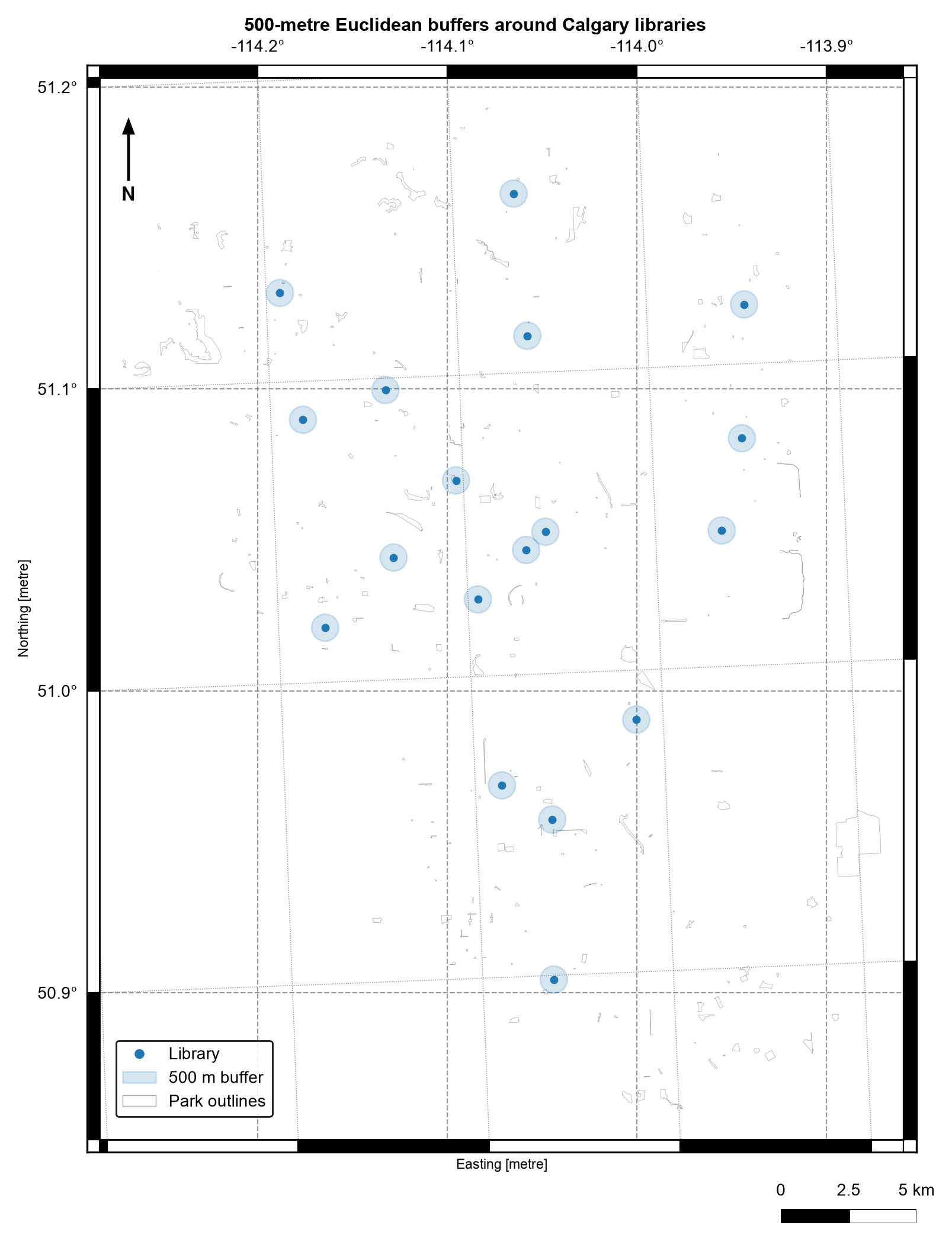
Fig. 4.5 500-metre Euclidean buffers around Calgary libraries over a sample of park outlines. Data: City of Calgary Open Data.

In Fig. 4.5, each zone is a small circle that stands apart from its neighbours, and large parts of the city lie outside every zone. The circles measure straight-line distance, so a library across a river or a rail line can fall inside a zone yet be far away by road.

4.2.9. Simplification and distance

representative_point() returns a point inside the feature, which makes it safer than centroid for labelling.

Simplification removes vertices while keeping the overall shape. GeoPandas uses the Douglas–Peucker algorithm [Douglas and Peucker, 1973], which drops a vertex when removing it moves the line by less than the tolerance. The tolerance is therefore the largest positional error you accept, in CRS units. preserve_topology=True prevents collapsed or self-crossing results at some cost in speed. Simplification changes measurements, since areas and lengths shrink, so use it for display and lighter files, never for the geometry you measure from.

Distance follows the rules in Table 4.10: it is Euclidean and measured to the nearest part of the other geometry, so like a buffer it is a crow-flies answer and not a route.

Show code cell source

Hide code cell source

circle = Point(0, 0).buffer(500)   # 64 vertices, radius 500 m

print(f'{"tolerance (m)":>14} {"vertices":>9} {"area change":>12}')
for tolerance in [0, 5, 25, 100]:
    simple = circle.simplify(tolerance, preserve_topology=True)
    change = simple.area / circle.area - 1
    print(f'{tolerance:>14} {len(simple.exterior.coords) - 1:>9} {change:>12.1%}')

 tolerance (m)  vertices  area change
             0        64         0.0%
             5        32        -0.5%
            25        16        -2.4%
           100         8        -9.8%

Halving the vertex count (64 to 32) with a 5 m tolerance costs only 0.5% of the area, but a 100 m tolerance leaves eight vertices and removes 9.8%. The 5 m tolerance used for the park display geometry is a choice about acceptable positional error, and it applies to the display column only.

Show code cell source

Hide code cell source

parks_m['label_point'] = parks_m.geometry.representative_point()
parks_m['display_geometry'] = parks_m.geometry.simplify(
    tolerance=5, preserve_topology=True
)

origin = libraries_m.geometry.iloc[0]
parks_m['distance_to_first_library_m'] = parks_m.geometry.distance(origin)

print(parks_m[['site_name', 'distance_to_first_library_m']].nsmallest(
    5, 'distance_to_first_library_m'
))
print('label points inside source:',
      parks_m['label_point'].within(parks_m.geometry).mean())

# Simplification must not create invalid or empty geometries.
assert parks_m['display_geometry'].notna().all()
assert parks_m['display_geometry'].is_valid.all()

                          site_name  distance_to_first_library_m
156                   OLYMPIC PLAZA                    84.795052
89                       PAGET PARK                   102.550583
60   JACK AND JEAN LESLIE RIVERWALK                   389.344509
460                    HARMONY PARK                   389.406005
169  JACK AND JEAN LESLIE RIVERWALK                   452.006811
label points inside source: 1.0

All label points fall inside their parks (100%), against 91.6% for centroids, which is the reason to prefer the representative point for labels. The nearest park to the first library is Olympic Plaza at 85 m, then Paget Park at 103 m; these are straight-line distances. The Jack and Jean Leslie Riverwalk appears twice in the list, so a park name is not a unique key.

4.2.10. Check what an operation returns

Every operation should be followed by a check of its output type, units, and plausible range, because a wrong CRS or a silent type change still returns a number or a geometry. Table 4.12 lists what to expect.

Table 4.12 Expected output and a quick check for each operation.

Operation	Returns	Units	Quick check
area, length, distance	Number per row	CRS units, squared for area	Not negative, and a plausible size in hectares or kilometres
envelope	Polygon	CRS units	Covers the source geometry
centroid	Point	CRS units	May lie outside the source, so count how often
convex_hull	Polygon, or a point or line for degenerate input	CRS units	Covers the source geometry
representative_point	Point	CRS units	Always within the source
buffer	Polygon or MultiPolygon	CRS units	A positive distance enlarges the area
simplify	Same type, fewer vertices	CRS units	Valid and not empty

The assert statements in the cells above apply these checks.

4.2.11. Performance and spatial indexes

Pairwise geometric questions scale badly: comparing every park against every library is an \(O(n \times m)\) operation. A spatial index avoids most of that work in two steps, called filter and refine. The index, a packed R-tree [Guttman, 1984, Leutenegger et al., 1997] in GeoPandas, groups nearby bounding boxes into a tree, so a query returns only the features whose boxes overlap the query box (the filter). The exact geometry test then runs on those candidates alone (the refine). A bounding box is only a rough outline, so the filter can return false candidates but never misses a true match.

This is why gpd.sjoin, gpd.sjoin_nearest, and the GeoPandas predicate accessors are preferred over Python loops. The index is also available directly as layer.sindex.query().

The cell below answers “which library is nearest to each park label point?” twice: with a brute-force loop on a 50-park sample, and with the indexed sjoin_nearest. The sample is small enough that both finish instantly, so the check confirms that the two approaches agree. Only the indexed version stays practical as both layers grow.

Show code cell source

Hide code cell source

sample_centroids = parks_m.geometry.representative_point().head(50)

# Brute force: every point tested against every library.
slow_matches = []
for point in sample_centroids:
    distances = libraries_m.geometry.distance(point)
    slow_matches.append(libraries_m['Library'].iloc[distances.argmin()])

# Indexed: bounding-box candidates first, exact distances second.
fast_matches = gpd.sjoin_nearest(
    gpd.GeoDataFrame(geometry=sample_centroids, crs=metric_crs),
    libraries_m[['Library', 'geometry']],
    how='left',
)['Library']

print('brute-force and indexed results agree:',
      (pd.Series(slow_matches).to_numpy() == fast_matches.to_numpy()).all())

brute-force and indexed results agree: True

4.2.12. Summary

Geometric operations are meaningful only when their spatial interpretation matches the question. Measurements inherit the CRS units, so reproject to a projected CRS before measuring, and remember that buffers and distances are crow-flies answers, not routes. Each derived geometry summarizes a feature differently: the centroid can fall outside it, the representative point cannot, and simplification trades accuracy for lighter geometry. Preserve the source geometry when creating derived columns, use spatial indexes instead of pairwise loops, and validate geometry type, units, row counts, and plausible values. Continue with S03 to attach attributes using keys and spatial relationships.