Remark

Please be aware that these lecture notes are accessible online in an ‘early access’ format. They are actively being developed, and certain sections will be further enriched to provide a comprehensive understanding of the subject matter.

3.2. The ESRI Shapefile

3.2.1. Learning Objectives

By the end of this section, you should be able to:

• Explain what a Shapefile is, why it is a collection of files, and which components are mandatory.

• Describe the role of each component (.shp, .shx, .dbf, .prj, .cpg, and metadata files) and how geometry and attributes are linked.

• Download and unpack a real Shapefile and recognize what each unpacked file is.

• Read a Shapefile in Python with GeoPandas, and with a low-level library when you only need to inspect it.

• Recognize a multi-layer collection of Shapefiles.

• Load a Shapefile with GeoPandas, filter and reproject it, map it, and write it back out to see the format’s limitations first-hand.

• Identify the format’s core limitations (field-name length, size, null handling, single geometry type, text types and encoding), explain why they matter, and apply a checklist after reading or writing one.

Section Goal

The Shapefile was introduced by ESRI in the early 1990s and remains ubiquitous in GIS despite its age and many limitations. You will meet it constantly in government and institutional data. This section is a self-contained lecture on the format: we start with a real download, take its files apart, read it in Python, and then catalog the limitations so you know exactly what to check before trusting a Shapefile’s contents.

3.2.2. What Is a Shapefile, and Why Does It Still Matter?

A Shapefile is a vector data format for storing the location and attributes of geographic features: points, lines, or polygons, each with a row of descriptive data. ESRI published its specification openly [ESRI, 1998], which allowed nearly every GIS tool to read and write it, and that openness is the main reason it became the default for exchanging vector data.

Its design reflects its era. It was built for desktop computers of the early 1990s: simple, fast to read, and split into several small files. That history explains both its strengths (universal support, easy to understand) and its weaknesses (the limits catalogued in Shapefile Format Limitations and Their Impacts). Today you will more often receive Shapefiles than choose them, so the practical skill is knowing how to read one safely.

3.2.3. Getting a Real Shapefile: US Census Counties

To keep the discussion concrete, we use the TIGER/Line county boundaries published by the US Census Bureau [Natural Earth contributors, n.d.].

1. Browse the TIGER/Line Shapefiles page.

2. Download the national counties file: tl_2023_us_county.zip.

3. Unzip it into a folder of your own, for example data/tl_2023_us_county/.

The resulting folder looks like this:

data/
  tl_2023_us_county/
    tl_2023_us_county.shp
    tl_2023_us_county.shx
    tl_2023_us_county.dbf
    tl_2023_us_county.prj
    tl_2023_us_county.cpg
    tl_2023_us_county.shp.iso.xml
    tl_2023_us_county.shp.ea.iso.xml

Notice that one dataset is seven files sharing a single base name. This is the first thing to understand about Shapefiles: when someone says “the Shapefile,” they mean the whole set.

Table 3.7 Files in an unpacked Shapefile download

Extension	Content	Status
.shp	Geometry (binary)	Mandatory
.shx	Geometry index: fixed-size records pointing into .shp	Mandatory
.dbf	Attribute table (dBASE format)	Mandatory
.prj	Coordinate reference system, written as WKT text	Optional, but essential in practice
.cpg	Character encoding declaration for the .dbf text	Optional, but strongly recommended
.shp.iso.xml	Dataset-level metadata (ISO 19115 format): title, publisher, dates, purpose	Optional
.shp.ea.iso.xml	Entity and attribute metadata: describes each field in the table	Optional

Three rules follow from this table:

• The three mandatory files are .shp, .shx, and .dbf. A Shapefile cannot be read without them.

• .prj and .cpg are optional by specification but not optional in practice. Without .prj, you do not know where the coordinates are on Earth. Without .cpg, text with accents or non-Latin characters may be misread.

• All files must share the same base name and stay in the same folder. Moving or renaming only the .shp breaks the dataset. Always copy, zip, and email the full set.

The two .xml files are metadata written by the publisher. They are easy to ignore, but they are where you find the data’s lineage and field definitions, the kind of documentation discussed in the later section on data sources.

The next cell does the downloading and unpacking in Python, so the notebook can be rerun on any machine. It downloads the archive only if the Shapefile is not already on disk, then lists what was unpacked, with each file’s size and whether it is mandatory.

Show code cell source

Hide code cell source

from pathlib import Path
import urllib.request
import zipfile

URL = "https://www2.census.gov/geo/tiger/TIGER2023/COUNTY/tl_2023_us_county.zip"
DATA_DIR = Path("data/tl_2023_us_county")
SHP = DATA_DIR / "tl_2023_us_county.shp"

# Download and unpack only if the Shapefile is not already on disk
if not SHP.exists():
    DATA_DIR.mkdir(parents=True, exist_ok=True)
    zip_path = DATA_DIR / "tl_2023_us_county.zip"
    request = urllib.request.Request(URL, headers={"User-Agent": "Mozilla/5.0"})
    with urllib.request.urlopen(request) as response, open(zip_path, "wb") as out_file:
        out_file.write(response.read())
    with zipfile.ZipFile(zip_path) as archive:
        archive.extractall(DATA_DIR)
    zip_path.unlink()          # keep only the Shapefile components

MANDATORY = {".shp", ".shx", ".dbf"}
print(f"Contents of {DATA_DIR}/")
for path in sorted(DATA_DIR.iterdir()):
    status = "mandatory" if path.suffix in MANDATORY else "optional"
    print(f"  {path.name:<34} {path.stat().st_size / 1e6:8.2f} MB   {status}")

Contents of data/tl_2023_us_county/
  tl_2023_us_county.cpg                  0.00 MB   optional
  tl_2023_us_county.dbf                  0.99 MB   mandatory
  tl_2023_us_county.prj                  0.00 MB   optional
  tl_2023_us_county.shp                131.40 MB   mandatory
  tl_2023_us_county.shp.ea.iso.xml       0.04 MB   optional
  tl_2023_us_county.shp.iso.xml          0.05 MB   optional
  tl_2023_us_county.shx                  0.03 MB   mandatory

One dataset, seven files, and almost all of the weight is in the geometry: the .shp is 131 MB, while the .dbf is under 1 MB and the .shx index only 0.03 MB, because it stores nothing but fixed-size pointers. The .prj and .cpg are a few bytes each, yet losing either would leave the coordinates or the text uninterpretable.

3.2.4. Anatomy: What Each Component Does

3.2.4.1. .shp, .shx, and .dbf: Three Files, One Table

The Shapefile stores geometry and attributes separately, and links them by position:

• .shp holds the shapes, one record per feature, in order.

• .dbf holds one row per feature, in the same order.

• .shx is an index into .shp that lets software jump directly to the n-th shape without scanning from the start.

So the 1st shape in .shp belongs to the 1st row in .dbf, the 2nd to the 2nd, and so on. There is no key column joining them. The consequence is practical: never sort, delete, or edit the .dbf on its own (for example by opening it in a spreadsheet and saving it). Doing so scrambles the match between shapes and their attributes without any error message.

When GeoPandas reads the set, it joins the two sides for you and gives a single table where each row has its attributes plus a geometry column.

3.2.4.2. .prj: The Coordinate Reference System

The .prj file describes the coordinate system in WKT (Well-Known Text), the same text notation family used for geometries. The TIGER/Line counties are in NAD83 geographic coordinates (EPSG:4269): longitude and latitude in degrees. This is close to, but not the same as, the WGS 84 system (EPSG:4326) used by GPS and web maps. The two differ by a small datum shift, which is why you should read the CRS from the data rather than assume. And because coordinates are degrees, distance or area computed directly on this layer is not in meters; reproject to a suitable projected CRS before measuring.

3.2.4.3. .cpg: Text Encoding

The .dbf stores text as bytes, and the .cpg states which character set those bytes use (commonly UTF-8). If it is missing or wrong, names such as “Doña Ana” can appear corrupted. When text looks garbled, suspect the encoding first.

3.2.4.4. Geometry Types in a Shapefile

A Shapefile holds exactly one geometry type: points, lines, or polygons (with variants for multipoints and for 3D or measured coordinates). Two details are worth knowing:

• Shapefile “lines” and “polygons” can contain multiple parts. A county made of separate pieces is still one record. When read into Python, the result may contain a mix of Polygon and MultiPolygon objects even though the file has just one “polygon” type. This is the same distinction that matters when loading into a spatial database.

• A single file cannot mix types. A dataset that logically needs points and polygons must be delivered as separate files.

3.2.4.5. Collections of Shapefiles (Multi-Layer Datasets)

Because one file holds one geometry type and one theme, datasets with several layers are delivered as a folder of several Shapefiles, each its own set of files with its own base name. Each Shapefile in the folder is a layer. For example, the Natural Earth cultural data [Natural Earth contributors, 2026] is published as separate downloads such as countries and states/provinces; unzipped into one folder, each becomes a layer you can list and open separately. This is a first glimpse of the “multi-layer container” idea that newer formats such as GeoPackage handle inside a single file.

3.2.5. Reading Shapefiles in Python

3.2.5.1. High-Level Access with GeoPandas

GeoPandas [Jordahl et al., 2020] is the right default for analysis. You give its read_file function the path to the .shp (for example, data/tl_2023_us_county/tl_2023_us_county.shp), and it finds the companion files by their shared base name, reads them as a set, and returns a GeoDataFrame: a table with one row per county and a geometry column.

Show code cell source

Hide code cell source

import geopandas as gpd
import pandas as pd

counties = gpd.read_file(SHP)          # GeoPandas finds .shx, .dbf, .prj, and .cpg by the shared base name
print(f"{len(counties):,} features, {counties.shape[1]} columns (including geometry)")
counties.head()

3,235 features, 19 columns (including geometry)

	STATEFP	COUNTYFP	COUNTYNS	GEOID	GEOIDFQ	NAME	NAMELSAD	LSAD	CLASSFP	MTFCC	CSAFP	CBSAFP	METDIVFP	FUNCSTAT	ALAND	AWATER	INTPTLAT	INTPTLON	geometry
0	31	039	00835841	31039	0500000US31039	Cuming	Cuming County	06	H1	G4020	NaN	NaN	NaN	A	1477563029	10772508	+41.9158651	-096.7885168	POLYGON ((-96.55516 41.91587, -96.55515 41.914...
1	53	069	01513275	53069	0500000US53069	Wahkiakum	Wahkiakum County	06	H1	G4020	NaN	NaN	NaN	A	680980771	61564427	+46.2946377	-123.4244583	POLYGON ((-123.72755 46.2645, -123.72756 46.26...
2	35	011	00933054	35011	0500000US35011	De Baca	De Baca County	06	H1	G4020	NaN	NaN	NaN	A	6016818946	29090018	+34.3592729	-104.3686961	POLYGON ((-104.89337 34.08894, -104.89337 34.0...
3	31	109	00835876	31109	0500000US31109	Lancaster	Lancaster County	06	H1	G4020	339	30700	NaN	A	2169269688	22850324	+40.7835474	-096.6886584	POLYGON ((-96.68493 40.5233, -96.69219 40.5231...
4	31	129	00835886	31129	0500000US31129	Nuckolls	Nuckolls County	06	H1	G4020	NaN	NaN	NaN	A	1489645187	1718484	+40.1764918	-098.0468422	POLYGON ((-98.2737 40.1184, -98.27374 40.1224,...

The layer has 3,235 rows, one for each county or county equivalent, and 19 columns: the 18 .dbf fields plus the geometry built from the .shp. The fields include (among others):

Table 3.8 County GeoDataFrame Field Descriptions and Examples

Field	Meaning	Example
STATEFP	State FIPS code	29 (Missouri)
COUNTYFP	County FIPS code within the state	019 (Boone County)
GEOID	State plus county code, a unique ID	29019
NAME, NAMELSAD	County name; name with legal/statistical description	Boone; Boone County
ALAND, AWATER	Land and water area, in square meters	numeric
INTPTLAT, INTPTLON	Internal point (representative location)	text
geometry	The county’s polygon	MultiPolygon or Polygon

Two lessons are hidden in this table:

• Codes are text, not numbers. FIPS codes like 019 have leading zeros. Stored as numbers they would become 19 and joins to other datasets would fail. The Census Bureau stores them as text, and so should you.

• Field names are 10 characters or fewer. NAMELSAD, INTPTLAT, and COUNTYNS all fit. Careful publishers design names to fit this limit; Shapefile Format Limitations and Their Impacts explains why.

The next cell checks both lessons directly. It shows how the codes are stored, and why GEOID, not NAME, is the key: several states have a Boone County.

Show code cell source

Hide code cell source

# Codes are stored as text, so leading zeros survive
print(counties[["STATEFP", "COUNTYFP", "GEOID"]].dtypes)
print()

# Converting a code to a number destroys the leading zeros
print("As text  :", counties["COUNTYFP"].head(3).tolist())
print("As number:", counties["COUNTYFP"].astype(int).head(3).tolist())
print()

# Names repeat across states; GEOID does not
print("NAME is unique :", counties["NAME"].is_unique)
print("GEOID is unique:", counties["GEOID"].is_unique)
counties.loc[counties["NAME"] == "Boone", ["STATEFP", "COUNTYFP", "GEOID", "NAME", "NAMELSAD"]]

STATEFP     str
COUNTYFP    str
GEOID       str
dtype: object

As text  : ['039', '069', '011']
As number: [39, 69, 11]

NAME is unique : False
GEOID is unique: True

	STATEFP	COUNTYFP	GEOID	NAME	NAMELSAD
329	54	005	54005	Boone	Boone County
507	29	019	29019	Boone	Boone County
1252	31	011	31011	Boone	Boone County
1573	21	015	21015	Boone	Boone County
1742	05	009	05009	Boone	Boone County
1954	17	007	17007	Boone	Boone County
1985	19	015	19015	Boone	Boone County
2155	18	011	18011	Boone	Boone County

Eight states have a Boone County, so NAME cannot serve as a key (False), while GEOID, which prefixes the state code, is unique. The cast to a number turns '039' into 39: the leading zero is lost, and joins against datasets that keep codes as text would silently fail.

3.2.5.2. Reading Only Part of a File

You can also read only part of a file, such as selected columns, a row range, or only features inside a bounding box. For a large national layer, this is much faster than loading everything.

Show code cell source

Hide code cell source

# Selected columns only (geometry is always included)
slim = gpd.read_file(SHP, engine="pyogrio", columns=["GEOID", "NAME", "ALAND"])

# Only features matching an attribute filter (SQL-style); here, Missouri (FIPS 29)
missouri_only = gpd.read_file(SHP, engine="pyogrio", where="STATEFP = '29'")

# Only features that intersect a bounding box: (min lon, min lat, max lon, max lat)
columbia_area = gpd.read_file(SHP, bbox=(-93.0, 38.5, -92.0, 39.5))

# Only the first few rows
first_rows = gpd.read_file(SHP, rows=5)

print(f"All columns : {counties.shape[1]}   Selected columns : {slim.shape[1]}")
print(f"All rows    : {len(counties):,}   Missouri : {len(missouri_only)}   "
      f"Bounding box : {len(columbia_area)}   First rows : {len(first_rows)}")

All columns : 19   Selected columns : 4
All rows    : 3,235   Missouri : 115   Bounding box : 13   First rows : 5

Filtering at read time returns only what was requested: four of the 19 columns, the 115 Missouri features (114 counties plus St. Louis city), the 13 counties that intersect the box around Columbia, and the first five rows.

3.2.5.3. Seeing the Position Link

Recall that the .shp and .dbf are matched by position, with no key joining them. The next cell shows what that means by shuffling the attribute rows and reattaching them to the unchanged geometries. Nothing fails; every row still looks fine. But the names no longer belong to their shapes.

Show code cell source

Hide code cell source

attributes = counties.drop(columns="geometry")                       # the .dbf side
shuffled = attributes.sample(frac=1, random_state=42).reset_index(drop=True)   # same rows, scrambled order

broken = gpd.GeoDataFrame(shuffled, geometry=counties.geometry.values, crs=counties.crs)

pd.DataFrame({
    "correct name": counties["NAME"].head(5).values,
    "name after shuffle": broken["NAME"].head(5).values,
})

	correct name	name after shuffle
0	Cuming	Oconto
1	Wahkiakum	Wabasha
2	De Baca	Forsyth
3	Lancaster	Sargent
4	Nuckolls	Fairfield

Cuming County’s polygon now carries the name Oconto, Wahkiakum’s carries Wabasha, and so on. Every row is individually plausible and no error is raised, which is why the .dbf must never be edited or re-sorted separately from the .shp.

3.2.5.4. Low-Level Access: Inspect Before You Load

Libraries such as Fiona (and pyogrio, which recent GeoPandas versions use by default) provide direct access to the same files. A low-level view is useful when you want to:

• list the layers in a folder before choosing one;

• check metadata (driver, CRS, schema, feature count) without reading all geometry; or

• stream a very large file one feature at a time instead of holding it all in memory.

Show code cell source

Hide code cell source

import pyogrio
import fiona
from collections import Counter

# pyogrio: quick metadata without reading any geometry
print("Layers in the folder:", pyogrio.list_layers(DATA_DIR).tolist())
info = pyogrio.read_info(SHP)
print("Driver    :", info["driver"])
print("CRS       :", info["crs"])
print("Features  :", f"{info['features']:,}")
print("Geometry  :", info["geometry_type"])
print("Encoding  :", info["encoding"])
print("Fields    :", list(info["fields"]))
print()

# Fiona: stream features one at a time instead of loading a table
with fiona.open(SHP) as src:
    print("Fiona sees:", src.driver, src.crs, f"{len(src):,} features")
    type_counts = Counter(feature["geometry"]["type"] for feature in src)
print("Geometry types in the file:", dict(type_counts))

Layers in the folder: [['tl_2023_us_county', 'Polygon']]
Driver    : ESRI Shapefile
CRS       : EPSG:4269
Features  : 3,235
Geometry  : Polygon
Encoding  : UTF-8
Fields    : ['STATEFP', 'COUNTYFP', 'COUNTYNS', 'GEOID', 'GEOIDFQ', 'NAME', 'NAMELSAD', 'LSAD', 'CLASSFP', 'MTFCC', 'CSAFP', 'CBSAFP', 'METDIVFP', 'FUNCSTAT', 'ALAND', 'AWATER', 'INTPTLAT', 'INTPTLON']

Fiona sees: ESRI Shapefile EPSG:4269 3,235 features
Geometry types in the file: {'Polygon': 3182, 'MultiPolygon': 53}

pyogrio and Fiona agree: EPSG:4269, 3,235 features, and UTF-8 text encoding read from the .cpg. The geometry counts show the multi-part point from earlier: although the layer is reported as Polygon, 53 of its features are MultiPolygon, because the single Shapefile polygon type holds both.

Table 3.9 Comparison of High-Level vs. Low-Level Spatial Data Access Tasks

Task	Use
Quick look at CRS, schema, and feature count; list layers	Low-level library (Fiona / pyogrio)
Stream a file too big for memory	Low-level library
Filter, join, plot, reproject, export as a table	GeoPandas

The usual workflow is to inspect first (what is in this folder, what CRS, how many features, which fields) and then load with GeoPandas once you know what you are getting.

3.2.6. Exploring and Visualizing a Shapefile

Reading a file is only the beginning. Maps are the fastest way to find problems and to see patterns, so we now look at the data we loaded.

3.2.6.1. Look Before You Analyze

The layer holds every county and county equivalent, including Alaska, Hawaii, and the island territories. Because some territories lie on opposite sides of the 180° meridian, a default map of the whole layer is stretched across the globe. A first plot like this is a quality check: it immediately shows scope and extent. Filtering on STATEFP gives us the contiguous United States.

Show code cell source

Hide code cell source

# FIPS codes of Alaska, Hawaii, and the island territories
NON_CONUS = ["02", "15", "60", "66", "69", "72", "78"]
conus = counties[~counties["STATEFP"].isin(NON_CONUS)].copy()
print(f"{len(counties):,} features in the layer, {len(conus):,} in the contiguous US")

3,235 features in the layer, 3,109 in the contiguous US

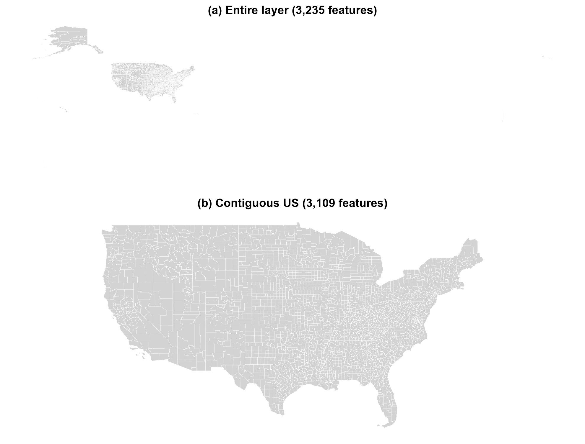
Fig. 3.5 The entire counties layer (a) and the contiguous United States after filtering on STATEFP (b).

Fig. 3.5 shows the scope check at work. In panel (a) the mainland is a small block in the upper left, because the westernmost Aleutian Islands and the Pacific territories lie in the Eastern Hemisphere and stretch the plot extent across nearly the whole globe. Removing seven state codes (126 features) gives the usable map in panel (b). The same filter-then-plot habit applies to any layer with outlying features.

3.2.6.2. Reproject Before You Measure

The layer is in NAD83 degrees. Degrees are angles, not lengths, so a one-degree square covers far less ground near the poles than at the equator. For maps and measurements of the contiguous US, an equal-area projection [Snyder, 1987] such as NAD83 / Conus Albers (EPSG:5070) is a better choice: it preserves areas and uses meters.

The first cell compares the two maps. The second shows the measurement consequence: area computed directly on the degree-based geometry is in square degrees, which is not a usable area, while the projected area should agree closely with the Census Bureau’s own ALAND + AWATER fields.

Show code cell source

Hide code cell source

conus_albers = conus.to_crs(epsg=5070)
print(f"CRS: {conus.crs} -> {conus_albers.crs}")

CRS: EPSG:4269 -> EPSG:5070

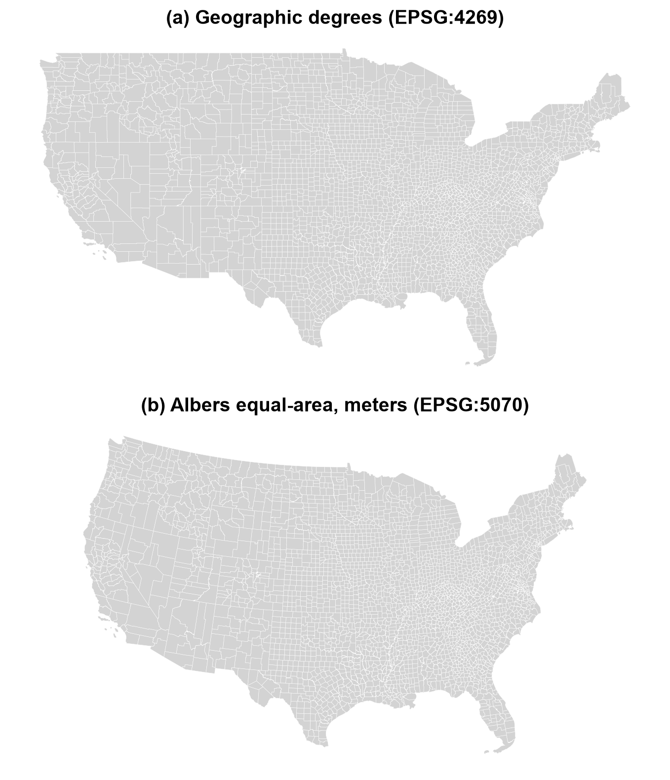
Fig. 3.6 Contiguous US counties in geographic degrees (a) and in the Albers equal-area projection (b).

The two maps in Fig. 3.6 hold the same data and differ only in CRS. In degrees (a), longitude and latitude are drawn as a flat grid, so the northern border is a straight line and the country looks stretched sideways. In the Albers projection (b), the border curves and the familiar shape appears, with areas preserved so that counties can be compared fairly.

Show code cell source

Hide code cell source

import warnings

with warnings.catch_warnings():
    warnings.simplefilter("ignore")            # GeoPandas warns that areas in degrees are not meaningful
    area_degrees = conus.geometry.area         # square DEGREES

area_km2 = conus_albers.geometry.area / 1e6                        # projected, converted to km2
reported_km2 = (conus["ALAND"] + conus["AWATER"]) / 1e6            # the Census Bureau's own figures

comparison = pd.DataFrame({
    "STATEFP": conus["STATEFP"],
    "NAME": conus["NAME"],
    "area in degrees^2 (not an area)": area_degrees.round(3),
    "projected area (km2)": area_km2.round(1),
    "ALAND + AWATER (km2)": reported_km2.round(1),
})
display(comparison[(comparison["STATEFP"] == "29") & (comparison["NAME"] == "Boone")])

ratio = area_km2 / reported_km2
print("Projected area / reported area (should be close to 1):")
print(ratio.describe().round(4))

	STATEFP	NAME	area in degrees^2 (not an area)	projected area (km2)	ALAND + AWATER (km2)
507	29	Boone	0.186	1789.8	1789.8

Projected area / reported area (should be close to 1):
count    3109.0
mean        1.0
std         0.0
min         1.0
25%         1.0
50%         1.0
75%         1.0
max         1.0
dtype: float64

For Boone County, the projected area (1,789.8 km²) matches the Census Bureau’s own ALAND + AWATER figure, while the same geometry in degrees gives 0.186, which is square degrees, not an area. Across all 3,109 contiguous counties the ratio of projected to reported area is 1.0 to four decimals, so the projection and the published figures agree.

3.2.6.3. Mapping an Attribute: Water Share

A choropleth colors each polygon by a value. Here the value is the share of each county’s area that is water, AWATER / (ALAND + AWATER), which highlights counties on the Great Lakes, along the coasts, and in wetland regions.

To make the map easier to read, we also derive state boundaries from the counties themselves. Dissolving merges all counties with the same STATEFP into one polygon per state and sums their land and water areas, so no separate state file is needed.

Show code cell source

Hide code cell source

conus_albers["water_share"] = conus_albers["AWATER"] / (conus_albers["ALAND"] + conus_albers["AWATER"])

states = conus_albers.dissolve(by="STATEFP", aggfunc={"ALAND": "sum", "AWATER": "sum"}).reset_index()
print(f"{len(conus_albers):,} counties dissolved into {len(states)} state-level polygons")

3,109 counties dissolved into 49 state-level polygons

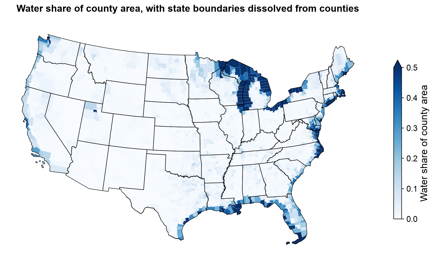
Fig. 3.7 Water share of county area for the contiguous US, with state boundaries dissolved from the counties.

In Fig. 3.7, the water share is high where county boundaries extend over open water. The Great Lakes counties of Michigan and Wisconsin saturate the scale (everything above 0.5 shares the darkest blue), followed by the Gulf Coast in Louisiana and Florida, the Chesapeake Bay and Atlantic coast, and Puget Sound. Most of the interior is almost white. The 49 dissolved state polygons (48 states plus the District of Columbia) give the map its frame without a separate state file.

3.2.6.4. Zooming In: Missouri and Boone County

Filtering to one state shows how attribute filtering and drawing work together. Missouri has 114 counties plus the independent city of St. Louis. The cell below highlights Boone County and overlays every county’s internal point.

INTPTLAT and INTPTLON are stored as text, so we convert them to numbers and build point geometries from them. This is a small example of constructing geometry from coordinate columns, a task you will meet often with tabular data.

Show code cell source

Hide code cell source

missouri = counties[counties["STATEFP"] == "29"].copy()
boone = missouri[missouri["NAME"] == "Boone"]

# Internal points are stored as text such as "+38.9..." -> convert, then build geometry
lon = pd.to_numeric(missouri["INTPTLON"])
lat = pd.to_numeric(missouri["INTPTLAT"])
internal_points = gpd.GeoSeries(gpd.points_from_xy(lon, lat), crs=missouri.crs)
print(f"{len(missouri)} Missouri features, {len(internal_points)} internal points built from text columns")

115 Missouri features, 115 internal points built from text columns

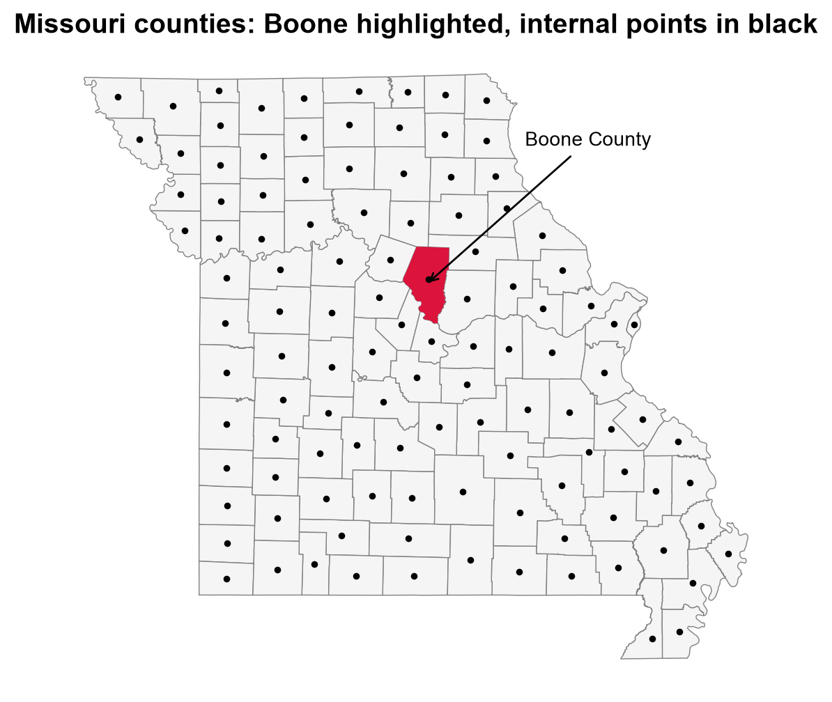
Fig. 3.8 Missouri counties with Boone County highlighted and each county’s internal point in black.

Boone County sits in the middle of the state in Fig. 3.8. Each county has exactly one black dot, and every dot falls inside its own polygon. That is a useful check on the conversion: had the text columns been misread, or longitude and latitude swapped, dots would land outside the state.

3.2.6.5. Ranking and Summarizing

Because the layer is a table, ordinary table operations apply. Sorting by land area, for example, shows which counties are largest. The area fields are in square meters, so we convert to square kilometers first.

Show code cell source

Hide code cell source

(counties
    .assign(land_km2=(counties["ALAND"] / 1e6).round(0))
    .nlargest(5, "land_km2")[["STATEFP", "NAME", "NAMELSAD", "land_km2"]])

	STATEFP	NAME	NAMELSAD	land_km2
520	02	Yukon-Koyukuk	Yukon-Koyukuk Census Area	377055.0
2246	02	North Slope	North Slope Borough	230052.0
1511	02	Bethel	Bethel Census Area	105253.0
242	02	Northwest Arctic	Northwest Arctic Borough	92367.0
1276	02	Southeast Fairbanks	Southeast Fairbanks Census Area	64315.0

All five largest counties are Alaskan boroughs or census areas, a reminder that “county equivalents” differ widely in kind and size. Rankings and averages over the whole layer therefore mix unlike units.

3.2.7. Putting It Together: A Safe Reading Routine

After reading any Shapefile, run a short set of checks before analysis:

Table 3.10 Safe Reading Routine Checks for Shapefiles

Check	What it tells you	In the counties example
Feature count	Whether the data loaded completely	Roughly 3,200 counties
Field names and types	Truncation; codes stored as numbers	GEOID should be text
CRS	Where coordinates are, and in what units	NAD83 degrees (EPSG:4269)
Geometry types	Single or mixed Polygon/MultiPolygon	Both may appear
Null or invalid geometries	Records that will break spatial operations	Should be none or few
Encoding	Whether text reads correctly	Names with accents look right

Making this routine a habit pays off whenever a Shapefile arrives from an unfamiliar source.

The function below turns this table into a reusable audit. Run it immediately after every read, before any analysis.

Show code cell source

Hide code cell source

def audit_shapefile(gdf, shp_path):
    """Print the checks from the safe reading routine for a GeoDataFrame read from a Shapefile."""
    cpg = Path(shp_path).with_suffix(".cpg")
    geom = gdf.geometry
    fields = [c for c in gdf.columns if c != geom.name]
    text_fields = [c for c in fields if pd.api.types.is_string_dtype(gdf[c])]

    print(f"Feature count      : {len(gdf):,}")
    print(f"Fields             : {len(fields)} (longest name: {max(len(c) for c in fields)} characters)")
    print(f"Text fields        : {len(text_fields)} of {len(fields)}")
    print(f"CRS                : {gdf.crs}")
    print(f"Geometry types     : {geom.geom_type.value_counts().to_dict()}")
    print(f"Null geometries    : {geom.isna().sum()}")
    print(f"Empty geometries   : {geom.is_empty.sum()}")
    print(f"Invalid geometries : {(~geom.dropna().is_valid).sum()}")
    print(f"Encoding (.cpg)    : {cpg.read_text().strip() if cpg.exists() else 'missing'}")

audit_shapefile(counties, SHP)

# Dataset-specific checks for this layer
print()
print("GEOID is unique    :", counties["GEOID"].is_unique)
print("GEOID is 5 chars   :", counties["GEOID"].str.len().eq(5).all())
print("Non-ASCII names    :", counties.loc[~counties["NAME"].str.isascii(), "NAME"].head(5).tolist())

Feature count      : 3,235
Fields             : 18 (longest name: 8 characters)
Text fields        : 16 of 18
CRS                : EPSG:4269
Geometry types     : {'Polygon': 3182, 'MultiPolygon': 53}
Null geometries    : 0
Empty geometries   : 0
Invalid geometries : 0
Encoding (.cpg)    : UTF-8

GEOID is unique    : True
GEOID is 5 chars   : True
Non-ASCII names    : ['Mayagüez', 'Canóvanas', 'Guánica', 'Doña Ana', 'Peñuelas']

The audit is clean: no null, empty, or invalid geometries; 18 fields with a longest name of 8 characters, inside the 10-character limit; EPSG:4269; and a UTF-8 .cpg. Names such as Doña Ana and Mayagüez read correctly, which confirms the encoding. A clean audit is evidence that the file is well formed, not proof that positions are accurate or attributes current.

3.2.8. Key Limitations

Most Shapefile problems are silent: the file opens, the map draws, and the error is still there. Know the limits and what each one does:

Table 3.11 Shapefile Format Limitations and Their Impacts

Limitation	What happens	Why it matters
10-character field names	Longer names are truncated when writing	Information is lost, and two long names can collapse into the same short one
2 GB limit per component (.shp, .dbf)	Large datasets cannot be stored in one Shapefile	Big layers must be split or stored in another format
No reliable null for numbers	Writers substitute zero or another placeholder	A real zero and a missing value become indistinguishable
One geometry type per file	Mixed data needs several files	Datasets turn into folders of files
Date only, no time	Timestamps cannot be stored in a date field	Time of day must be stored as text or in extra fields
Limited text and number types	Text fields are capped at 254 characters; few data types	Long descriptions get cut off
Weak Unicode handling	Special characters corrupt without a correct .cpg	Names and places appear garbled
Multi-file fragility	Components separate or get renamed	A missing .shx, .dbf, or .prj breaks or degrades the dataset

3.2.8.1. Worked Example: Field-Name Truncation

Suppose a table has a column called CrimeDescriptionAndLocation. That name is 27 characters long. When written to a Shapefile, it is silently cut to its first 10 characters, CrimeDescr, with no error (GeoPandas prints a warning that is easy to miss, and other tools may say nothing). If the table also has CrimeDescriptionOnly, both names now begin CrimeDescr, and the writer must invent a new name for one of them; GDAL produces CrimeDes_1 [GDAL/OGR contributors, 2026]. The lesson is to choose short, meaningful field names before exporting, and always reopen the written file and compare field names against the original.

The next cell writes a small table to a Shapefile and reads it back. Besides the field names, it includes a 300-character text value and a timestamp, so you can see two more limits at work.

Show code cell source

Hide code cell source

import tempfile
import warnings
from shapely.geometry import Point, box


def write_and_report(gdf, path, **kwargs):
    """Write a file and print any warnings raised along the way (shortened for readability)."""
    with warnings.catch_warnings(record=True) as caught:
        warnings.simplefilter("always")
        gdf.to_file(path, **kwargs)
    for item in caught:
        print("  warning:", str(item.message)[:95])


demo = gpd.GeoDataFrame(
    {
        "CrimeDescriptionAndLocation": ["theft near campus"],
        "CrimeDescriptionOnly": ["theft"],
        "Notes": ["long note " * 30],
        "ReportedAt": pd.to_datetime(["2026-10-16 14:30:00"]),
    },
    geometry=[Point(-92.33, 38.95)],
    crs="EPSG:4326",
)

with tempfile.TemporaryDirectory() as folder:
    demo_path = Path(folder) / "demo.shp"
    print("Writing the Shapefile...")
    write_and_report(demo, demo_path)
    back = gpd.read_file(demo_path)
print()

print("Field names before:", [c for c in demo.columns if c != "geometry"])
print("Field names after :", [c for c in back.columns if c != "geometry"])
print("Text length before/after:", len(demo.loc[0, "Notes"]), "->", len(back.loc[0, "Notes"]))
print("Timestamp before/after  :", demo.loc[0, "ReportedAt"], "->", back.loc[0, "ReportedAt"],
      f"(stored as {back['ReportedAt'].dtype})")

Writing the Shapefile...
  warning: Column names longer than 10 characters will be truncated when saved to ESRI Shapefile.
  warning: Normalized/laundered field name: 'CrimeDescriptionAndLocation' to 'CrimeDescr'
  warning: Normalized/laundered field name: 'CrimeDescriptionOnly' to 'CrimeDes_1'
  warning: Field ReportedAt created as String field, though DateTime requested.
  warning: Value 'long note long note long note long note long note long note long note long note long not

Field names before: ['CrimeDescriptionAndLocation', 'CrimeDescriptionOnly', 'Notes', 'ReportedAt']
Field names after : ['CrimeDescr', 'CrimeDes_1', 'Notes', 'ReportedAt']
Text length before/after: 300 -> 254
Timestamp before/after  : 2026-10-16 14:30:00 -> 2026/10/16 14:30:00 (stored as str)

One write caused four silent losses. Both long column names were cut to ten characters and, because they began alike, the second received a _1 suffix to stay unique. The 300-character note was cut to 254. The timestamp came back as the string 2026/10/16 14:30:00, because the DBF has a date type but no time of day. Warnings were raised, but nothing failed, which is why reopening the written file matters.

A single Shapefile also cannot hold mixed geometry types. Trying to write a point and a polygon into the same file fails:

Show code cell source

Hide code cell source

mixed = gpd.GeoDataFrame(
    {"id": [1, 2]},
    geometry=[Point(-92.33, 38.95), box(-93.0, 38.0, -92.0, 39.0)],
    crs="EPSG:4326",
)

with tempfile.TemporaryDirectory() as folder:
    try:
        mixed.to_file(Path(folder) / "mixed.shp")
    except Exception as error:
        print(f"{type(error).__name__}: {error}")

FeatureError: Could not add feature to layer at index 1: Attempt to write non-point (POLYGON) geometry to point shapefile.

Unlike the losses above, this limit is enforced with an explicit error.

3.2.8.2. Living with the Format

Despite these limitations, Shapefile remains the format you are most likely to receive from government agencies, so working with its constraints is indispensable. A sensible policy:

• Receiving: read it, run the checks in Safe Reading Routine Checks for Shapefiles, and keep the original untouched.

• Working: for repeated analysis, convert to a modern format that removes most of these limits (the next section introduces one).

• Delivering: provide Shapefile only when the recipient requires it, with short field names, a .prj, and a .cpg, and verify the output by reading it back.

To see the difference, the cell below writes the same Missouri table to both formats. It adds one column with a long, descriptive name, then compares the files produced and the field names that survive.

Show code cell source

Hide code cell source

missouri_demo = missouri[["NAME", "geometry"]].assign(land_area_square_meters=missouri["ALAND"])

with tempfile.TemporaryDirectory() as folder:
    folder = Path(folder)
    print("Writing the Shapefile...")
    write_and_report(missouri_demo, folder / "missouri.shp")
    write_and_report(missouri_demo, folder / "missouri.gpkg", driver="GPKG")
    print()

    shp_files = sorted(p.name for p in folder.glob("missouri.*") if p.suffix != ".gpkg")
    print("Shapefile  files :", shp_files)
    print("Shapefile  fields:", [c for c in gpd.read_file(folder / "missouri.shp").columns if c != "geometry"])
    print()
    print("GeoPackage files :", sorted(p.name for p in folder.glob("*.gpkg")))
    print("GeoPackage fields:", [c for c in gpd.read_file(folder / "missouri.gpkg").columns if c != "geometry"])

Writing the Shapefile...
  warning: Column names longer than 10 characters will be truncated when saved to ESRI Shapefile.
  warning: Normalized/laundered field name: 'land_area_square_meters' to 'land_area_'

Shapefile  files : ['missouri.cpg', 'missouri.dbf', 'missouri.prj', 'missouri.shp', 'missouri.shx']
Shapefile  fields: ['NAME', 'land_area_']

GeoPackage files : ['missouri.gpkg']
GeoPackage fields: ['NAME', 'land_area_square_meters']

The Shapefile shortened land_area_square_meters to land_area_ and produced five files, while the GeoPackage kept the full name in a single file.

Practice

Download and unzip tl_2023_us_county.zip into data/tl_2023_us_county/. List the files, mark which are mandatory, and read the layer with GeoPandas. Then record the feature count, CRS, geometry types, and field names, and note which field would break if it were treated as a number. Then pick a state other than Missouri, map its counties colored by land area, and save the result as a GeoPackage.

3.2.9. Key Terms

Table 3.12 Key Terms for Shapefile Concepts

Term	Meaning
Shapefile	A multi-file vector format from ESRI storing geometry and attributes.
.shp / .shx / .dbf	The three mandatory files: geometry, geometry index, attribute table.
.prj	File holding the coordinate reference system in WKT.
.cpg	File declaring the text encoding of the attribute table.
dBASE (DBF)	The legacy table format used for Shapefile attributes.
Layer	One Shapefile in a folder of several; one geometry type and theme.
FIPS code	A numeric-looking standard identifier for states and counties, best stored as text.
NAD83 (EPSG:4269)	The geographic coordinate system used by TIGER/Line data.
Truncation	Silent cutting of a field name beyond 10 characters.

3.2.10. Review Questions

1. Which three files must exist for a Shapefile to be readable, and what does each hold?

2. How are geometries in the .shp linked to rows in the .dbf, and why is editing the .dbf alone dangerous?

3. The .prj of the counties layer says NAD83 degrees. What does that imply for computing county areas directly from the geometry?

4. Why should COUNTYFP and GEOID be stored as text?

5. A field named PopulationEstimate2020 is exported to a Shapefile. What happens, and how would you detect it?

6. When would you inspect a Shapefile with a low-level library instead of loading it with GeoPandas?

3.2.11. Summary

A Shapefile is a set of files that must stay together: .shp, .shx, and .dbf are mandatory, and .prj and .cpg (plus metadata XML) are optional by specification but essential in practice. Geometry and attributes are stored separately and matched by position. The format’s single-geometry-type rule, 10-character field names, 2 GB limit, weak null and text handling, and fragility as a multi-file bundle trace back to the 1990s, and they can silently corrupt data if unchecked. GeoPandas is the practical default for analysis, while low-level libraries support inspection and streaming. Because Shapefile remains common in legacy and government data, always re-verify field names, geometry, CRS, and encoding immediately after reading one.

The next section introduces two modern, multi-layer alternatives that remove most of these limitations: GeoPackage and the Esri File Geodatabase.