Remark
Please be aware that these lecture notes are accessible online in an ‘early access’ format. They are actively being developed, and certain sections will be further enriched to provide a comprehensive understanding of the subject matter.
3.8. Lab: Utilizing rasterio package with Raster Data Model Example#
3.8.1. Setting Up the Environment#
Before we begin our analysis, we need to import the necessary libraries. These libraries are essential for handling raster data and performing GIS operations in Python:
numpy: This fundamental package for scientific computing provides support for large, multi-dimensional arrays and matrices. In raster analysis, numpy is crucial for handling the grid-based structure of raster data and performing numerical operations on pixel values.
rasterio: This library provides a powerful interface for reading and writing raster datasets. Built on top of GDAL, rasterio offers Pythonic access to geospatial raster data, including:
Reading and writing various raster formats
Handling coordinate reference systems
Performing raster operations and transformations
matplotlib: This comprehensive library for creating static, animated, and interactive visualizations includes:
pyplot: The main plotting interface
colors: Tools for color mapping and manipulation
patches: Objects for adding shapes to plots
rasterio.plot: An extension of rasterio that provides specialized plotting functions for raster data visualization.
rasterio.warp: Provides tools for coordinate transformations and reprojection of raster data.
These libraries work together seamlessly:
numpy handles the numerical operations and array management
rasterio provides the core raster data functionality
matplotlib creates the visualizations
rasterio’s extensions add specialized geospatial capabilities
Package |
Description |
Documentation |
|---|---|---|
Scientific computing with arrays |
||
Geospatial raster data access |
||
Comprehensive plotting library |
This combination of libraries provides a robust framework for working with raster data, from basic file operations to complex spatial analysis and visualization.
3.8.2. Understanding Our Data#
For this lab, we’ll be working with two different types of satellite data products obtained from Google Earth Engine (GEE). A more detailed exploration of remote sensing concepts, including the theoretical foundations and practical applications.
3.8.2.1. MODIS Land Cover (MCD12Q1)#
The MCD12Q1_LC_Type4_500m_2023.tif is a MODIS (Moderate Resolution Imaging Spectroradiometer) Land Cover Type product. This dataset is derived from combined Terra and Aqua satellite observations and demonstrates how raster data can represent discrete, categorical information:
Purpose: Represents land cover as discrete categories, where each pixel value corresponds to a specific land cover type. The classification is derived using supervised classifications of MODIS Terra and Aqua reflectance data.
Spatial Resolution: 500 meters
Temporal Coverage: 2001-2023 annual composites
Classification Scheme: Type 4 (BIOME-BGC), one of five different classification schemes (IGBP, UMD, LAI, BGC, and PFT)
Data Type: 8-bit unsigned integer, with values ranging from 0 to 8, fill value of 255
Description: Provides a discrete classification of global land cover types using supervised classifications that undergo additional post-processing incorporating prior knowledge and ancillary information to refine specific classes
Let’s visualize this dataset first:
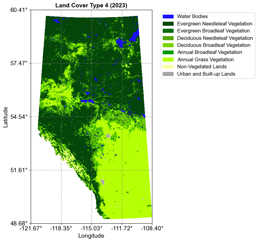
This visualization demonstrates how categorical raster data can be effectively displayed using distinct colors for each land cover class, making it easy to interpret different landscape features.
3.8.2.2. MODIS NDVI (MOD13A1)#
The MOD13A1_NDVI_20230610.tif is a Terra MODIS Vegetation Index product that provides continuous measurements of vegetation health and density:
Purpose: Provides Vegetation Index (VI) values computed from atmospherically corrected bi-directional surface reflectances that have been masked for water, clouds, heavy aerosols, and cloud shadows
Spatial Resolution: 500 meters
Temporal Coverage: 16-day composite (product available from 2000-02-18)
Data Type: 16-bit signed integer with scale factor 0.0001
Valid range: -2000 to 10000
Scaled NDVI values range from -0.2 to 1.0
Description: NDVI is referred to as the continuity index to the existing NOAA-AVHRR derived NDVI:
NDVI = (NIR - RED)/(NIR + RED)
Uses red (645nm) and NIR (858nm) bands
Higher values indicate denser vegetation
Lower values indicate sparse vegetation
Quality Assurance: Includes DetailedQA and SummaryQA bands for assessing data quality
Let’s visualize this dataset:
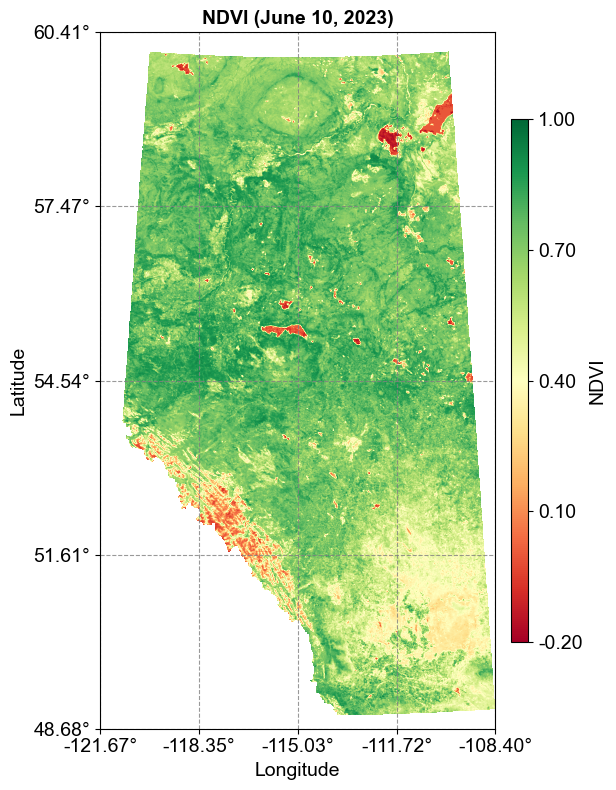
This visualization uses a Red-Yellow-Green (RdYlGn) color scheme where:
Red represents low NDVI values (sparse vegetation)
Yellow represents moderate NDVI values
Green represents high NDVI values (dense, healthy vegetation)
The continuous color gradient reflects the nature of NDVI as a quantitative measurement, in contrast to the discrete categories of the land cover classification.
3.8.2.3. Dataset Comparison and Visualization#
The MCD12Q1 and NDVI datasets demonstrate two fundamental ways that raster data can represent geographic information:
Categorical vs. Continuous Data:
MCD12Q1 (Land Cover):
Represents discrete, categorical data
Each pixel contains one of 9 possible values
Values are qualitative, representing distinct land cover types
Visualized using a discrete color scheme where each class has a unique color
NDVI:
Represents continuous, quantitative data
Values range continuously from -0.2 to 1.0 (stored as -2000 to 10000)
Values indicate vegetation density and health
Visualized using a continuous color gradient (RdYlGn)
Visualization Approach To effectively display these different data types, we employ distinct visualization strategies:
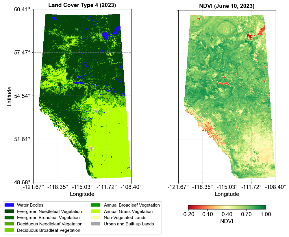
Key visualization considerations:
Layout: Side-by-side comparison using subplots with shared y-axis
Color Schemes:
Land Cover: Discrete colors with a legend showing class names
NDVI: Continuous color gradient with a calibrated colorbar
Legend Types:
Land Cover: Categorical legend with patches for each class
NDVI: Continuous colorbar with scaled values
Spatial Reference:
Both plots maintain equal aspect ratios
Coordinates are transformed to geographic (lat/lon) for consistency
Shared latitude axis ensures proper spatial alignment