Attribute and Spatial Joins

4.3. Attribute and Spatial Joins#

4.3.1. Learning objectives#

By the end of this section, you should be able to:

distinguish a relational join from a spatial join;
describe key cardinality, and declare and validate it with validate=;
preserve identifier types so keys actually match;
explain what gpd.sjoin returns: its rows, columns, and index;
explain the left, right, and inner join modes of gpd.sjoin;
choose a spatial predicate such as within or intersects deliberately;
report unmatched and duplicated records; and
aggregate joined results without double-counting features.

Section goal

Join Calgary library records to a small lookup table, then locate libraries inside community districts. The left-hand layer remains the unit of analysis, so every change in row count has to be explainable.

4.3.2. Two kinds of matching#

An attribute join [Codd, 1970] compares values in columns, such as a branch identifier or postal prefix. A spatial join compares geometries, such as a point being within a district. Both families raise the same row-semantics question: which input controls the retained records, and can one row match many? Table 4.13 summarizes the three join modes.

Table 4.13 Join modes, the rows each retains, and their typical use.#
Mode	Rows retained	Typical use
`how='left'`	Every left row; unmatched right columns are null	Keep the unit of analysis complete
`how='right'`	Every right row; unmatched left columns are null	Inventory the right layer
`how='inner'`	Only rows with a match on both sides	Analyze matched pairs only

how='left' means that the left layer controls which records are retained; it does not mean that every record must find a match. Spatial joins can also be one-to-many: a point on a shared boundary may match more than one polygon with intersects, and overlapping polygons can duplicate a left feature. Use a unique identifier and an explicit aggregation rule when counting.

4.3.3. Keys and cardinality#

An attribute join pairs rows whose key values are equal. Two properties of the keys decide whether the result can be trusted.

The first is cardinality: how many rows on each side may share one key value. Table 4.14 lists the four cases and the matching validate= argument of DataFrame.merge [McKinney, 2010].

Table 4.14 Join cardinality and the *validate=* value that enforces it.#
Relationship	Key is unique on	Example	`validate=`
One to one	Both sides	A district and its row in a count table	`'one_to_one'`
Many to one	The right side only	Branches looked up in a postal-area table	`'many_to_one'`
One to many	The left side only	A district and the libraries inside it	`'one_to_many'`
Many to many	Neither side	Rarely intended; it multiplies rows	`'many_to_many'` (no check)

A many-to-one lookup is the usual design. When the lookup accidentally holds a duplicate key, each matching left row is copied once per duplicate, which is called fan-out, and every later count is inflated. Declaring the expected relationship makes pandas raise an error instead of continuing quietly.

The second property is the key type and form. Values must match exactly: '0' is not 0, and 'T2G ' is not 'T2G'. pandas refuses to merge an integer key with a text key, but a trailing space or a case difference simply fails to match, and the rows fall out as nulls in a left join or disappear in an inner join. Normalize keys (text type, stripped, one case) before merging. The toy tables below show each failure.

left  merge: 5 rows from 4 branches
inner merge: 4 rows from 4 branches
MergeError: Merge keys are not unique in right dataset; not a many-to-one merge
ValueError: You are trying to merge on int64 and str columns for key 'key'

The left merge turns four branches into five rows because the lookup repeats T2J. The inner merge returns four rows only by coincidence: it drops Nose Hill, which has no match, and duplicates Fish Creek, so the two errors cancel. An unchanged row count does not prove a clean join, which is why the declared validate= check and the unmatched count both matter.

4.3.4. Load the layers#

The next cell loads the library and community layers [Open Calgary: The City of Calgary Open Data Portal, 2026] with the same parsing as S01, keeps a stable branch_id and community_id, and derives the three-character postal area used as the join key below.

libraries: 18 communities: 313

4.3.5. Attribute join with declared cardinality#

The lookup below is derived from the library table only to keep this notebook reproducible; in a real project it could be a separately maintained table. Each postal_area occurs once in the lookup, so many library rows may match one lookup row: many_to_one is the intended relationship. Declaring it with validate= turns a silent fan-out mistake into an explicit error. Every postal area here happens to hold a single branch, so each looked-up count is 1; the point is the declared relationship and the unchanged row count, not the values.

                         Library postal_area  branches_in_postal_area
 W.R. Castell Central Library         T2G                        1
    Alexander Calhoun Library         T2T                        1
              Bowness Library         T3B                        1
           Fish Creek Library         T2J                        1
          Forest Lawn Library         T2A                        1
      Glenmore Square Library         T2C                        1
         Louise Riley Library         T2N                        1
        Memorial Park Library         T2R                        1
            Nose Hill Library         T2L                        1
            Shawnessy Library         T2Y                        1
         Signal Hill Library         T3H                        1
           Southwood Library         T2W                        1
       Judith Umbach Library         T2K                        1
      Village Square Library         T1Y                        1
            Crowfoot Library         T3G                        1
       Country Hills Library         T3K                        1
         Saddletowne Library         T3J                        1
           Westbrook Library         T3C                        1

4.3.6. How a spatial join works#

A spatial join replaces the key comparison with a predicate: two rows are matched when the stated relationship between their geometries holds, using the relationships from S01. gpd.sjoin(left, right, how=, predicate=) [Jordahl et al., 2020] follows the filter and refine steps from S02: a spatial index [Guttman, 1984, Leutenegger et al., 1997] on the right layer finds candidate pairs by bounding box, and the exact predicate then runs on those candidates.

The result has a predictable shape:

Rows: one row per matching pair. A left row with k matches appears k times, and one with no match appears once with null right columns in a left join, or not at all in an inner join.
Columns: every left column, then the right columns, plus index_right, the row label of the matching right feature. Clashing names receive _left and _right suffixes. A left or inner join keeps the left geometry; a right join keeps the right geometry.
Index: a left join keeps the left index, so a repeated index label marks a fan-out.

Unlike merge, sjoin has no validate= argument, so row counts, duplicated identifiers, and unmatched rows must be checked by hand. A predicate is also all-or-nothing: a point just outside a polygon, because of a digitising gap or a coastline, is unmatched, not assigned to the nearest polygon. gpd.sjoin_nearest, used in S02, assigns the nearest match when that is the rule you actually want.

Four toy points and three toy districts make the rules visible. Point p2 sits on the edge shared by districts A and B, p4 is outside every district, and district C holds no point.

left  within      rows=4
inner within      rows=2
right within      rows=3
left  intersects  rows=5

  point_id  index_right district
0       p1          0.0        A
1       p2          0.0        A
1       p2          1.0        B
2       p3          1.0        B
3       p4          NaN      NaN

With within, p2 is unmatched because it lies on the boundary, not in the interior of either district, and p4 is unmatched because it lies outside all of them; the inner join drops both, and the right join keeps district C although no point reached it. With intersects, p2 matches both A and B, so four points produce five rows and the index label 1 appears twice. The predicate is therefore a decision about boundary contact. For a rule that assigns every point to exactly one district, within and intersects both need a tie-break, such as keeping the first match or using sjoin_nearest.

4.3.7. Spatial join: libraries within community districts#

The library points are the left layer and the district polygons are the right layer. The predicate is the analytical choice, and Table 4.15 lists the options.

Table 4.15 Spatial predicates for joins, when each matches, and what to use it for.#
Predicate	Matches when	Use it for
`within`	the left geometry is inside the right geometry, excluding its boundary	Assigning points to exactly one district
`intersects`	the geometries share any point, including the boundary	Cases where boundary contact should count
`contains`	the left geometry contains the right geometry	Polygon-first questions, with polygons as the left layer
`dwithin`	the geometries are within `distance=` of each other	Proximity joins in a projected CRS

A point that lies exactly on a polygon boundary is not within it [Herring, 2011]; use intersects when boundary contact should count. Both layers are already in EPSG:4326, but a CRS comparison should still be part of a reusable workflow.

output rows: 18
unmatched libraries: 0
duplicate branch matches: 0
                        Library                      NAME
0  W.R. Castell Central Library  DOWNTOWN COMMERCIAL CORE
1     Alexander Calhoun Library             SOUTH CALGARY
2               Bowness Library                   BOWNESS
3            Fish Creek Library               WILLOW PARK
4           Forest Lawn Library               FOREST LAWN

All 18 libraries land in exactly one district, with no unmatched rows and no duplicate matches. A branch’s name need not match its district’s: Fish Creek Library sits in Willow Park and the Alexander Calhoun Library in South Calgary, so the assignment comes from geometry, not from names.

4.3.8. Compare join modes and predicates#

Running the same layers under the three join modes exposes what each one preserves. An inner join drops unmatched left rows without any warning, which is why a left join is the safer default when the left layer is the unit of analysis. Comparing within with intersects shows how boundary contact changes the result.

left rows:    18 (every library kept)
inner rows:   18 (unmatched libraries dropped)
right rows:  313 (every district kept)
districts with no library: 295
extra boundary matches from intersects: 0

In this dataset every library falls inside exactly one district, so the inner join keeps all 18 rows and intersects adds no matches. The right join shows the other side: 295 of the 313 districts contain no library. With other layers, the same code can drop or duplicate left rows, which is why the counts are worth printing.

4.3.9. Aggregate without double-counting#

Counting after a join means choosing the unit being counted. size() counts joined rows, whereas nunique() on an identifier counts distinct features. The two agree only when no fan-out occurred. In the toy join above, each district’s count is correct on its own, because p2 really does touch both A and B, but adding the district counts together counts p2 twice.

joined rows: 5
rows per district: {'A': 2, 'B': 2}
sum of district counts: 4
distinct points matched: 3

4.3.9.1. Library counts by district#

A count should name its unit. Here the unit is a library branch, not a row in the joined result. nunique() protects the count if a later predicate or an overlapping district layer produces several matches for one branch. A left merge followed by fillna(0) then gives every district an explicit zero when no library was assigned. The map after the checks shows the resulting counts by district.

count    313.000000
mean       0.057508
std        0.233183
min        0.000000
25%        0.000000
50%        0.000000
75%        0.000000
max        1.000000
Name: library_count, dtype: float64

The mean of 0.0575 is simply 18 districts out of 313 (5.75%), and the median, quartiles, and minimum are all 0, so this count is dominated by zeros. A district average of 0.06 libraries is a poor summary of such a layer, and the map or a table of the 18 districts says more.

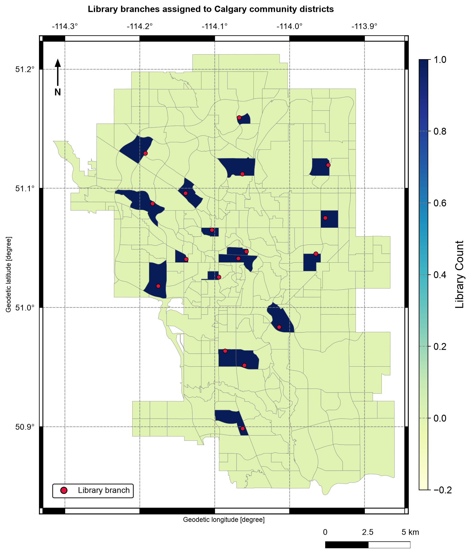
../_images/join_library_counts.png — Fig. 4.6 Number of library branches assigned to each Calgary community district by a left spatial join with the `within` predicate. Data: City of Calgary Open Data.#

In Fig. 4.6, 18 districts are shaded dark because each holds one library, while the other 295 are pale because they hold none. Every black point lies inside a dark district, which is what the within join found. The legend runs continuously from 0 to 1 even though a count here is only ever 0 or 1, so read the map as two classes.

4.3.10. Common pitfalls#

Silent fan-out: a duplicated key or overlapping right polygons multiply left rows. Check branch_id.duplicated().sum() after every join.
Dropped rows: inner joins and dropna() remove records without reporting them. Print unmatched counts before aggregating.
Mismatched key types: a postal code read as an integer in one table and text in another will not match. Normalize key types first.
Near-miss keys: trailing spaces and case differences do not raise an error; they appear as nulls after a left join.
Boundary points: within leaves them unmatched and intersects matches them to every polygon they touch. Choose a rule deliberately.
No built-in check on sjoin: it has no validate=, so compare row counts and duplicated identifiers yourself.
Degree-based distance joins: dwithin uses CRS units, so run it in a projected CRS when the threshold is in metres.
Counting the wrong column: count unique branch identifiers, not joined rows.

4.3.11. Summary#

Attribute joins use keys; spatial joins use predicates. Choose the join mode from the layer that must be preserved, declare the expected cardinality, preserve a stable identifier, normalize key types, align CRSs, and report unmatched or duplicated rows before aggregating. A spatial join returns one row per matching pair, so boundary contact and overlapping polygons can multiply left rows, and counts should name their unit. Continue with S04 for operations that split and combine areas.