1.1. Systems of Equations, Geometry

Linear Equation

A linear equation in two variables is an algebraic expression of the form

(1.1)\[\begin{align} ax+by = c \end{align}\]

where \(a\), \(b\), and \(c\) are constants, and \(a\) and \(b\) are not both zero. The constants \(a\) and \(b\) determine the slope and direction of the line, while the constant \(c\) determines its position on the coordinate plane. This equation describes a set of points \((x, y)\) that lie on a straight line. Any point \((x, y)\) that satisfies the equation is a solution of the equation, and any solution of the equation is a point on the line.

Linear equations and their graphs are important topics in mathematics. They have many applications in different fields, such as modeling real-world situations, finding solutions to systems of equations, and studying geometric shapes and transformations. A linear equation in two variables is an algebraic expression that relates two variables with a constant term. The graph of a linear equation is a straight line that shows all the possible values of the variables that satisfy the equation. The slope and intercept of the line depend on the coefficients and constant of the equation. By understanding how to manipulate and interpret linear equations and their graphs, one can explore various mathematical concepts and problems [Kuttler and Farah, 2020, Nicholson, 2018].

For example, \(x-y=0\) is a linear equation.

Note that, in this example, \(x\) and \(y\) are the variables. However, in general, when more than two variables are involved, variables are often denoted with some subscripts. For example, \(x_1\), \(x_2\), …, \(x_n\) are variables for an equation of the form [Kuttler and Farah, 2020, Nicholson, 2018]

(1.2)\[\begin{align} a_1 x_1 +a_2 x_2 +\ldots+a_n x_n = b \end{align}\]

where \(a_1\), \(a_2\), …, \(a_n\) and \(b\) are constants. Moreover, \(\Sigma\) (Sigma) is often used to represent a sum of some terms. For example, the equation above can also be written as follows

(1.3)\[\begin{align} \sum_{j = 1}^{n} a_j\,x_j = b. \end{align}\]

This is also known as summation notation or sigma notation. It is a convenient way to write a sum of \(n\) terms, where \(j\) is the index of summation that varies from \(1\) to \(n\). The symbol \(\sum\) indicates the sum, and the terms \(a_j\,x_j\) are added together. Summation notation can be used to simplify and generalize expressions involving sums [Kuttler and Farah, 2020, Nicholson, 2018].

System of Linear Equations

A system of equations is a collection of equations that involve the same variables. For example, the following \(m\) equations form a system of (linear) equations:

(1.4)\[\begin{align} \begin{cases} a_{11}x_1 + \ldots + a_{1n}x_n = b_1 \\ a_{21}x_1 + \ldots + a_{2n}x_n = b_2 \\ \vdots \\ a_{m1}x_1 + \ldots + a_{mn}x_n = b_m \\ \end{cases} \end{align}\]

In this system, there are \(m\) equations and \(n\) variables, \(x_1, x_2, \ldots, x_n\). Each equation contains a linear combination of these variables with coefficients \(a_{ij}\), and the right-hand side of each equation is given by \(b_i\). A system of equations can be used to model various situations where multiple relationships between variables are given. For example, a system of equations can represent the supply and demand of a product, the balance of chemical reactions, or the intersection of geometric figures. The main goal of solving a system of equations is to find the values of the variables that satisfy all the equations simultaneously. These values are called the solutions of the system. There are different methods to solve a system of equations, such as substitution, elimination, or matrix operations [Kuttler and Farah, 2020, Nicholson, 2018].

Solving a system of equations involves finding the values of the variables \(x_1, x_2, \ldots, x_n\) that make all the equations in the system true at the same time. The solution to the system is the set of values for the variables that satisfy each equation [Kuttler and Farah, 2020, Nicholson, 2018].

Systems of equations have many applications in various fields, such as engineering, physics, economics, and optimization problems. They are essential for understanding and modeling complex relationships and interactions between different variables in real-world scenarios [Kuttler and Farah, 2020, Nicholson, 2018].

Using summation notation, the given linear equation can be written as [Kuttler and Farah, 2020, Nicholson, 2018]:

(1.5)\[\begin{align} \sum_{j=1}^{n} a_{ij}x_{j} = b_i, \quad i = 1, 2, 3, \ldots, m. \end{align}\]

In this notation, \(i\) is the index of each equation in the system (from 1 to \(m\)), while \(j\) is the index of each variable (from 1 to \(n\)). The coefficients \(a_{ij}\) and the variables \(x_j\) are multiplied and added together in the summation on the left-hand side of each equation. The right-hand side of each equation is given by \(b_i\).

Summation notation is a useful mathematical tool that allows us to represent a system of linear equations with multiple variables and equations in a concise way. It simplifies the expression and makes it easier to manipulate and solve complex systems of equations.

Example: The following system of equations,

\[\begin{align*} \begin{cases} x_1-2x_2-7x_3=7\\ -x_1+3x_2+6x_3=25\pi \end{cases}\end{align*}\]

is linear because each equation has the form

\[\begin{align*} a_1x_1 + a_2x_2 + \ldots + a_nx_n = b \end{align*}\]

where \(a_1, a_2, \ldots, a_n\) and \(b\) are constants, and \(x_1, x_2, \ldots, x_n\) are variables. A linear equation has no terms that involve products, powers, or roots of the variables.

This system of equations has

• Variables (unknowns): \(x_1, x_2\) and \(x_3\). These are the quantities that we want to find by solving the system. They are also called the dependent variables because their values depend on the coefficients and constants of the system.

• Coefficients (the first equation): \(1, -2\), \(-7\). These are the constants that multiply the variables in the first equation. They are also called the independent variables because their values do not depend on the variables of the system.

• Coefficients (the second equation): \(-1, 3\), \(6\). These are the constants that multiply the variables in the second equation. They are also called the independent variables because their values do not depend on the variables of the system.

• Constant term (the first equation): \(7\). This is the constant that is added or subtracted from the linear combination of the variables in the first equation. It is also called the right-hand side of the first equation because it is on the right side of the equal sign.

• Constant term (the second equation): \(25\pi\). This is the constant that is added or subtracted from the linear combination of the variables in the second equation. It is also called the right-hand side of the second equation because it is on the right side of the equal sign.

Homogeneous System of Equations

A system of equations is called homogeneous if all the right-hand side values are zero. This means that each equation in the system is equal to zero. A homogeneous system has the following general form:

(1.6)\[\begin{align} a_{11}x_1 + a_{12}x_2 + \ldots + a_{1n}x_n &= 0 \\ a_{21}x_1 + a_{22}x_2 + \ldots + a_{2n}x_n &= 0 \\ &\vdots \\ a_{m1}x_1 + a_{m2}x_2 + \ldots + a_{mn}x_n &= 0 \\ \end{align}\]

where \(a_{ij}\) are the coefficients of the variables, and \(x_1, x_2, \ldots, x_n\) are the variables. The system has \(m\) equations and \(n\) variables. A homogeneous system always has at least one solution, which is the trivial solution where all the variables are zero. However, a homogeneous system may also have nontrivial solutions, where some or all of the variables are nonzero. Whether a homogeneous system has nontrivial solutions or not depends on the number and rank of the equations and the variables [Kuttler and Farah, 2020, Nicholson, 2018].

Homogeneous systems of equations are important in mathematics and its applications, as they can be used to study the properties and behavior of linear transformations, vector spaces, eigenvalues and eigenvectors, and differential equations [Kuttler and Farah, 2020, Nicholson, 2018].

Homogeneous systems of equations are of special interest in linear algebra and have important applications in various areas, such as linear transformations, eigenvalues, and eigenvectors. Solving homogeneous systems often involves finding non-trivial solutions, meaning solutions where not all variables are zero. The existence and properties of non-trivial solutions can reveal valuable insights into the behavior of certain mathematical structures and physical phenomena [Kuttler and Farah, 2020, Nicholson, 2018].

Example: The system of equations,

\[\begin{align*} \begin{cases} x+y=0\\ x-y=0,\\ \end{cases} \end{align*}\]

is homogeneous because all the right-hand side values are zero. This system has two equations and two variables, \(x\) and \(y\). The trivial solution of this system is \(x = y = 0\). However, this system also has non-trivial solutions, which can be found by solving one of the equations for one of the variables and substituting it into the other equation. For example, solving the first equation for \(x\), we get \(x = -y\). Substituting this into the second equation, we get \(-y - y = 0\), which implies that \(y = 0\). Therefore, any value of \(x\) that satisfies \(x = -y\) is a non-trivial solution of the system. In other words, the non-trivial solutions are of the form \((x, -x)\), where \(x\) is any nonzero number. These solutions form a line that passes through the origin and has a slope of \(-1\). This line is called the solution set of the system, and it represents all the possible values of \(x\) and \(y\) that make both equations true. The solution set of a homogeneous system is always a subspace of the vector space that contains the variables [Kuttler and Farah, 2020, Nicholson, 2018].

Solution of a Linear System

A solution for a linear system is a set of values for the variables that make all the equations in the system true at the same time. For example, if \((x_1, x_2, x_3, \ldots, x_n)\) is a solution for a linear system, it means that when we plug in these values into each equation of the system, we get a true statement. In other words, the solution satisfies every equation in the linear system. A solution can be verified by substituting the values of the variables into the equations and checking if they are equal to the right-hand side values. A linear system can have zero, one, or infinitely many solutions, depending on the number and rank of the equations and the variables [Kuttler and Farah, 2020, Nicholson, 2018]. Finding the solution or solutions of a linear system is one of the main goals of linear algebra. There are different methods to solve a linear system, such as substitution, elimination, or matrix operations [Kuttler and Farah, 2020, Nicholson, 2018].

Example: Show that \(x = -2\), \(y = 5\), \(z = 0\) and \(x = 0\), \(y = 4\), \(z = -1\) are both solutions to the system,

\[\begin{align*} \begin{cases} x+y+ z=3,\\ 2x+y+3z=1. \end{cases} \end{align*}\]

To show that a set of values for the variables is a solution to a system of equations, we need to substitute these values into each equation of the system and check if they satisfy the equations. In other words, we need to verify that the left-hand side and the right-hand side of each equation are equal after plugging in the values.

• Try \(x = -2,~y = 5,~z = 0\)

\[\begin{align*} \begin{cases} x+y+ z=3,\\ 2x+y+3z=1. \end{cases} \Rightarrow \begin{cases} (-2)+5+ 0=3\\ 2(-2)+5+3(0)=1 \end{cases} \Rightarrow \begin{cases} 3=3~\surd\\ 1=1~\surd \end{cases},\end{align*}\]

We see that both equations are true when we substitute \(x = -2,~y = 5,~z = 0\). Therefore, this is a solution to the system.

• Try \(x = 0,~y = 4,~z = -1\)

\[\begin{align*}\begin{cases} x+y+ z=3,\\ 2x+y+3z=1. \end{cases} \Rightarrow \begin{cases} 0+4+ (-1)=3\\ 2(0)+4+3(-1)=1 \end{cases} \Rightarrow \begin{cases} 3=3~\surd\\ 1=1~\surd \end{cases},\end{align*}\]

We see that both equations are true when we substitute \(x = 0,~y = 4,~z = -1\). Therefore, this is also a solution to the system.

We have shown that both sets of values are solutions to the system by verifying that they satisfy each equation in the system. A system of equations can have more than one solution, depending on the number and rank of the equations and the variables [Kuttler and Farah, 2020, Nicholson, 2018].

---

1.1.1. Possible sets of solutions for two equations and two variables

When a system of linear equations has only two variables, then the solutions to that system of linear equations can be explained geometrically using a graph. The graph of an equation \(ax+by = c\) is a straight line when \(a\) and \(b\) are not both zero at the same time [Kuttler and Farah, 2020, Nicholson, 2018].

For the following system of linear equations (with two variables), there are three possibilities.

(1.7)\[\begin{align} \begin{cases} a_{11}x+a_{12}y=b_1\\ a_{21}x+a_{22}y=b_2\\ \end{cases} \end{align}\]

1. The lines intersect at only one point. Then the system has a unique solution corresponding to that point.

Example: For the following system of linear equations,

\[\begin{align*} \begin{cases} x + y = 2\\ x - y = -1\\ \end{cases} \end{align*}\]

we have,

As can be seen, \((x, y) = (0.5, 1.5)\) is a solution. In this case, it’s the only solution (unique solution).

2. The lines are parallel (and distinct) and so do not intersect. Then the system has no solution.

Example: For the following system of linear equations,

\[\begin{align*} \begin{cases} x + y = 2\\ x + y = -1\\ \end{cases} \end{align*}\]

we have,

The two lines are parallel and there is no solution.

3. The lines are identical. Then the system has infinitely many solutions.

Example: For the following system of linear equations,

\[\begin{align*} \begin{cases} 2\,x + 2\,y = 2\\ x + y = 1\\ \end{cases} \end{align*}\]

we have,

1.1.2. Consistent and inconsistent linear systems

A system of equations is called inconsistent when there is no solution for this system of equations, and it is called consistent when there is at least one solution for it [Kuttler and Farah, 2020, Nicholson, 2018].

The graph of \(ax+by+cz = d\) (it has three variables) is a plane.

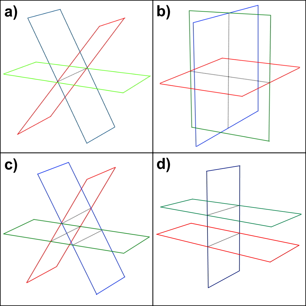
Fig. 1.1 a) three planes intersecting in a line, b) three planes intersecting in a point, c) three planes with no intersection, d) three planes with no intersection

This graphical method has its limitations. When more than three variables are involved, we cannot graph the planes anymore. However, we can still use algebraic methods to solve systems of equations with more than three variables, such as matrix operations or Gaussian elimination [Kuttler and Farah, 2020, Nicholson, 2018].